DOI:10.32604/iasc.2021.018405
| Intelligent Automation & Soft Computing DOI:10.32604/iasc.2021.018405 | |
| Article |
Feature Selection Using Artificial Immune Network: An Approach for Software Defect Prediction
1Faculty of Computing, Riphah International University, Islamabad, 45211, Pakistan
2Department of Computing and Informatics, Saudi Electronic University, Riyadh, 11673, Saudi Arabia
*Corresponding Author: Summrina Kanwal. Email: summrina@gmail.com
Received: 07 March 2021; Accepted: 12 April 2021
Abstract: Software Defect Prediction (SDP) is a dynamic research field in the software industry. A quality software product results in customer satisfaction. However, the higher the number of user requirements, the more complex will be the software, with a correspondingly higher probability of failure. SDP is a challenging task requiring smart algorithms that can estimate the quality of a software component before it is handed over to the end-user. In this paper, we propose a hybrid approach to address this particular issue. Our approach combines the feature selection capability of the Optimized Artificial Immune Networks (Opt-aiNet) algorithm with benchmark machine-learning classifiers for the better detection of bugs in software modules. Our proposed methodology was tested and validated using 5 open-source National Aeronautics and Space Administration (NASA) data sets from the PROMISE repository: CM1, KC2, JM1, KC1 and PC1. Results were reported in terms of accuracy level and of an AUC with highest accuracy, namely, 94.82%. The results of our experiments indicate that the detection capability of benchmark classifiers can be improved by incorporating Opt-aiNet as a feature selection (FS) method.
Keywords: Feature selection (FS); machine learning; optimized artificial immune networks (Opt-aiNet); software defect prediction (SDP); software metrics
The development industry has already established deep roots in almost all businesses and industries worldwide. Although software applications have improved the efficiency of business operations, the software development process is nevertheless complex and fraught with difficulties. The complexity of its software makes it failure-prone (full of faults/defects). According to IEEE standards, a fault, bug or defect is considered to be an inappropriate step, process or data in a computer program [1]. A software bug or defect results in software failure, something which occurs when the actual behavior differs from the intended functionality; in other words, there is inconsistency between the actual and the required functionality of the software [1]. To overcome these issues, a great deal of effort is required in terms of maintaining software quality (defect-free products) and ensuring user satisfaction. According to Zhang, a large number of software systems have many defects. According to the World Quality Report (WQR 2020), end-user satisfaction is now a top priority for Quality Assurance (QA) and testing. The report indicates that 27% of the total development cost was spent on testing and quality assurance and this is in fact expected to rise soon to 32% of the total information technology (IT) budget [2]. Over the past few years, numerous studies focusing on SDP models have been reported in the literature. SDP is a means of locating bugs in the software being developed so that the quality and productivity can be improved. Defect prediction models forecast the defective modules in software which are likely to be more error-prone in the future, and the models also help to determine the impact of these defective modules. The building of defect prediction models involves training a machine-learning model using software metrics to predict the defects in software units. Generally, the aim of these models is to forecast the software quality using a set of directly-measurable internal software metrics, such as size and complexity metrics [3]. Software metrics are called ‘features’ or ‘attributes’ that themselves are independent explanatory variables. The effectiveness of the trained model is directly dependent on the worth of these features. Extraneous and redundant features reduce the performance of the prediction models. The greater the number of features in the model, the greater is the complexity, and the less accurate is the model’s performance. To address this issue, we applied Opt-aiNet as an FS technique, in conjunction with benchmark machine-learning classifiers for a better prediction of software bugs. We experimented with six machine-learning classifiers, namely, a Support Vector Machine (SVM), a K-Nearest Neighbor (KNN), a Naive Bayesian (NB), a Decision Tree (DT), a Linear Discriminate Analysis (LDA) and a Random Forest (RF), and then presented the results in terms of accuracy.
FS is the process of selecting relevant features and eliminating noisy and less important features for model training. Our proposed technique reduces the model’s complexity and improves its prediction accuracy. Our proposed method identifies and selects a useful subset of the features which represent patterns from a larger set of mutually-redundant features with different associated measurement risks. To date, much work has been done in the field of SDP but, regrettably, the importance of FS for building consistent and highly-performing prediction models is often overlooked. Some of the prediction models are based on metrics computed using data taken from the change and defect history of software products to predict those components that are expected to be more error-prone than the others [3]. The performance of the SDP model is usually influenced by the characteristics of the attributes/features [4]. However, a set of standard features that can be used for defect prediction has yet to be finalized. The performance of these models increases if an FS technique is applied to eliminate the irrelevant features from the data set [5,6].
Recently, researchers have used different approaches, such as metrics (feature) based defect prediction, optimization schemes, machine-learning techniques and hybrid techniques (a combination of optimization and machine-learning). The field of metric-based defect prediction, which includes both filter and wrapper methods, is considered to be a promising technique for prediction purposes [7]. We believe that, although powerful prediction models have been proposed, there is nevertheless still room for improvement in the prediction quality of models. Therefore, organizations are still curious about methods or techniques that could improve the prediction quality of their models.
A number of models have been proposed to address the FS issue based on computational intelligence approaches, such as genetic algorithms (GA) Particle Swarm Optimization (PSO), Ant Colony Optimization (ACO), etc. [8]. Artificial Immune System (AIS), a sub-field of computational intelligence is emerging as one of the most promising approaches for solving complex computational or engineering problems [9]. Opt-aiNet is a biology-inspired algorithm from the AIS family and was first proposed by de Castro et al. [9]. Opt-aiNet consists of a network of antibodies that are similar to population in GA. It also has selection and mutation methods similar to those of GA. All Opt-aiNet, PSO and ACO have a memory set [9,10]. Besides having these, only Opt-aiNet has several additional features, which gave us the confidence to delve in deeper and use it for our research. The additional features are:
• Dynamically adjustable population size.
• Capability of maintaining many optimal solutions.
• Multiple Interactions.
• Exploration of the search space.
• Defined stopping criteria.
This has motivated us to continue exploring the field of Artificial Immune Networks (AIN) and contributing to the development of the new AIN models and techniques which are intended to more profoundly resolve the issue of early defect predictions. To the best of our knowledge, there has in fact been no published attempt to apply Opt-aiNet or its modified version to the SDP problem. Hence, in this study, we used a particular feature selection technique based on “Opt-aiNet” to improve the quality of the prediction model and to analyze its impact on the overall accuracy of defect prediction.
The rest of the paper is organized as follows: Section 2 presents a summary of the related work and the techniques used for SDP, Section 3 presents background information about the techniques used in this paper, and Section 4 explains the proposed method used while the whole experimental set-up is explained in Section 5 with the results being described in Section 6. Section 7 provides a comparison with previous techniques and a statistical analysis of our proposed technique while Section 8 concludes the paper with some final comments.
In this section, we discuss the previous work conducted by various researchers in the SDP field. It is evident that a great deal of effort has been dedicated in recent years to improving the prediction accuracy of SDP models. The performance of these models is primarily based on the following two main factors: the classifier(s) that is/are used in the modeling process and the quality of the data (the type and number of metrics) involved in the model-building process (FS) [11,12]. In this study, however, we are more concerned with the latter. FS is an important data preprocessing task in many data-mining and machine-learning applications. Chen et al. [13] investigated the use of wrapper-based feature selection methods in terms of software cost and effort estimation and concluded that a minimized set of data could actually improve the estimation of the cost/effort required. Khoshgoftaar et al. [14] were amongst the pioneers who conducted a comprehensive study based on the development of FS techniques for imbalanced data sets. In their study, they applied different wrapper-based feature-ranking and feature -subset selection techniques to generate candidate feature sets and different classification algorithms for prediction. The results showed an improved performance and indicated that if a better feature selection approach were to be applied, the SDP models could be enhanced and applied to real-case scenarios. Gao et al. [15] suggested a hybrid methodology involving a feature ranking for attribute selection, followed by the selection of a feature subset via an algorithm to get a final attribute subset. The study concluded that the selection of resilient features reduces the dimension, resulting in less time complexity with no detrimental effect on the performance of the overall model. Arar et al. [16] proposed a cost-sensitive Artificial Neural Network (ANN)-based ABC algorithm for SDP. In this study, features were selected using the WEKA tool with the help of a correlation-based FS technique. The researchers concluded that the reduction of the number of features had no significant effect on prediction accuracy. Xu et al. [17] compared the performance of 32 FS techniques when applied to both a noisy and a clean NASA data set. Wang et al. [18] proposed a Deep Belief Network (DBN) for feature extraction. In this technique, features are learned mechanically from token vectors extracted from the abstract syntax trees of a program. These extracted features are then used to train a defect prediction model. The execution of this model is then evaluated by comparing the extracted features with the traditional features. Li et al. [19] proposed an inspiring approach, known as the Defect Prediction via Convolutional Neural Network (DP-CNN), which utilized the concept of deep learning (DL) for effective feature generation. The token vectors are extracted from the abstract syntax tree (ASTs) of a program and are then encoded as numerical vectors via mapping and word-embedding. Furthermore, the semantic features of programs were mined using convolutional neural networks (CNN). All the extracted features were then combined and utilized for accurate SDP. Jayanthi et al. [20] applied a feature reduction approach, known as Principal Component Analysis (PCA). By incorporating maximum likelihood estimation for error, they reduced the likelihood of error in the construction of PCA features. Further, the selected features were fed to the neural network-based classification technique for bug prediction. Manjula et al. [21] presented a hybrid approach for bug prediction that combined a genetic algorithm (GA) for feature optimization with a deep neural network (DNN). A controlled experiment was performed using the MATLAB tool and the NASA open-source data set from the PROMISE repository. The DNN technique was incorporated using an adaptive auto-encoder for a better representation of selected features. The results from this study suggested that the improved performance of the proposed hybrid approach was a direct result of the deployment of optimization techniques. Xu et al. [22] proposed a new SDP framework called KPWE, that combined two techniques: a kernel principal component analysis (KPCA) and a weighted extreme learning machine (WELM), focusing on the feature extraction and class imbalance issues [23]. In this paper, an Opt-aiNet-based SDP model is proposed, one which uses several machine-learning classifiers for bug prediction. The parameters of these machine-learning classifiers were tuned to improve the bug prediction accuracy [23]. In this paper, three under-sampled methods were used for the decision region range, namely, a hybrid multi-objective cuckoo search for an under- sampled SDP model based on SVM (HMOCSUS-SVM). The HMOCS-US-SVM was proposed to solve simultaneously the problem of class imbalance (CIB) in data sets and the parameter selection of SVM.
Based on the various literature reviews of SDP problems .it was found that in most defect prediction studies feature selection techniques were not used or, if used, they only minimized the size of the data set without accessing the effects of feature selection on the overall accuracy of the defect prediction model. In contrast, our study aimed to introduce a model for software defect prediction using the AIN and machine-learning classifiers. The machine-learning classifiers were used in conjunction with the AIN to improve the prediction accuracy through feature selection. We also investigated the effect of feature selection on classifiers by comparing the prediction accuracy of these classifiers both before and after feature selection.
The technique proposed in this study evolved in two steps. Firstly, we selected resilient features using Opt-aiNet. Then, a number of machine learner classifiers, namely, SVM, KNN, NB, DT, LDA and RF, were applied for bug perdition. The results were reported in terms of prediction accuracy and AUC. The prediction accuracy results with and without FS were then compared to evaluate the performance of the machine-learning classifiers. The workflow for the proposed approach is shown in Fig. 1 below.
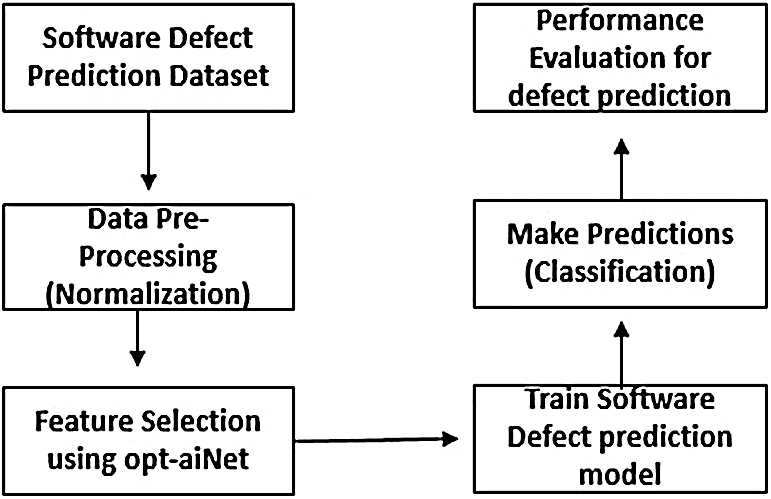
Figure 1: The overall workflow of the proposed approach
3.1 Optimized Artificial Immune Network (Opt-aiNet)
The artificial immune network algorithm (aiNet) was inspired by the immune network theory of the natural immune system [9–24]. The Opt-aiNet algorithm is an extension of the aiNet applied to solve optimization problems. There are in fact several modified versions of Opt-aiNet: Opt-aiNet for multi-modal optimization problems by de Castro et al. [7], Copt-aiNet for combinatorial optimization tasks by de Franca et al. [25], and Dopt-aiNet for Dynamic Optimization by Castro et al. [11,26]. In our study, we used Opt-aiNet, an optimization version of aiNet, which is a discrete immune network algorithm that produces a population by means of clonal expansion, mutation, selection and mutual interaction [27]. The population consists of a network of antibodies (candidate solutions to the function being optimized). The population is then evaluated according to objective function, clonal expansion, mutation, selection and interaction between themselves. Opt-aiNet creates a memory set of antibodies that represents (over time) the best candidate solutions to the objective function. Opt-aiNet is capable of both uni-modal and multi-modal optimization. The key terminologies that facilitate the understanding and implementation of Opt-aiNet are given below:
• Antigen: the desired/achieved target or solution.
• Network cell: a single unit (cell) in a population.
• Fitness: the value of the optimized objective function calculated for a particular cell.
• Affinity: the Euclidean distance between two cells.
• Clone: the offspring cells that are replicas of their parent cells which undergo cloning and mutation for variation from their ancestors.
The flow chart of the Opt-aiNet is shown in Fig. 2.
3.2 Machine-Learning Classifiers
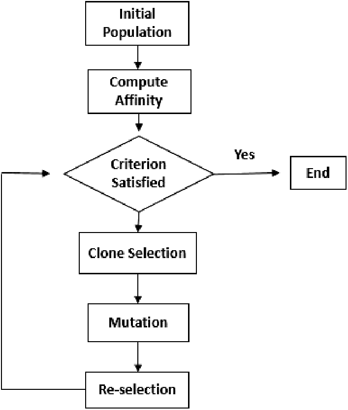
Figure 2: Flow chart of Opt-aiNet
The six classifiers implemented in this experiment are SVM, KNN, NB, DT, LDA and RF. These classifiers were selected as they are commonly applied within the software engineering domain, and because they have no in-built attribute (feature) selection capability, except for Discriminate Analysis, which, in this study, is used only as a classifier. Below is a brief introduction of these classifiers.
Cover et al. [28] of the Bell Laboratory introduced SVM in 1992. SVM defines the decision plane as a separation between a set of objects having different class memberships. In a high-dimensional feature space, the SVM algorithm uses a linear function to classify the sample data. Generally, two classification problems occur, one being the linear separable case and other being non-linear. In this study we have used the linear SVM. Linear SVM classifies the data that is linearly separable into two classes and a support vector machine is selected with a maximal margin due to its low generalization error [29,30].
The KNN algorithm is an instance-based learning method, also known as memory-based learning [31]. It is considered to be one of the simplest of all machine learning algorithms. The KNN works by finding the distances between two neighbors and then applying this to all the examples in the data by selecting a specified number of examples, such as, say K. K’ is a parameter that is the selection of the neighboring entities that will participate in the voting process. In a KNN algorithm, a test sample is assigned to the class of the majority of its nearest neighbors. In other and plainer words, if you are similar to your neighbors, then you are one of them. Similarity is defined according to the distance metric between two data points. A popular one is the Euclidean distance method.
where d is the distance function, n is the number of variables, xi and yi are the variables of vectors x and y respectively, in a two-dimensional vector space. i.e., x = (x1,x2,x3,. . .) and y = (y1,y2,y3,. . .).
NB is a probability-based classifier based on Bayes Theorem [32]. It works by determining the relationship between the probabilities of an event which is currently occurring with the probability of another event which has already occurred. The Bayes Theorem equation is:
In Eq. (2) above, P(c) and P(x) is the prior probability of class and predictor. P(c/x) is the posterior probability of the class (c, target) given predictor (x, attributes). P(x/c) is the likelihood, which is the probability of a predictor given class.
A Decision Tree (DT) is a supervised machine-learning algorithm mainly used for Regression and Classification [33]. It breaks down a data set into smaller and smaller subsets at the same time as an associated decision tree is incrementally developed. The data set will consist of attributes (sometimes referred to as features or characteristics) and a class attribute. The DT algorithm then builds a decision tree model. The model consists of a root node, branches and leaf nodes. The DT algorithm is a recursive algorithm, i.e., it calls itself and processes the data recursively until stopping criteria are met. This criterion is usually when the data runs out or if all examples in the subset belong to the same class, i.e., the examples have the same attribute value for the class attribute. The decision tree can handle both categorical and numerical data.
In LDA, a set of prediction equations are found, based on the independent variables that are used to classify each individual into a particular group [34]. LDA serves two purposes, namely, finding a predictive equation to classify new individuals, and interpreting the predictive equation that exists among the variables to have a better understanding of their relationship.
Random forest (RF) is a supervised machine-learning algorithm that creates a forest with a number of trees [35]. In RF, the number of trees is directly proportional to the resulting accuracy; that is to say, the greater the number of trees in the forest, the greater is the accuracy of the results. When creating a forest of trees, the RF first constructs each individual tree using bagging and feature randomness. To create decision tress, the RF first extracts subsamples from the original samples using the bootstrap method, and then secondly, the decision trees are classified to implement a simple vote, with the largest classification vote being the final result of the prediction. In the next section the proposed Opt-aiNet technique is described.
4 The Proposed Opt-aiNet as a FS Technique
FS is the technique of choosing useful features or eliminating unnecessary features/ attributes from the initial data, either by using some personal qualities of data or by evaluating the data with an optimized function [36]. The feature subset is selected in order to obtain a condensed feature set according to a certain optimization principle, which results in a better representation of the original data and with the best possible minimal set. We selected features using AIN. The workflow of Opt-aiNet is depicted in Fig. 3 and the steps taken are also described in more detail below.
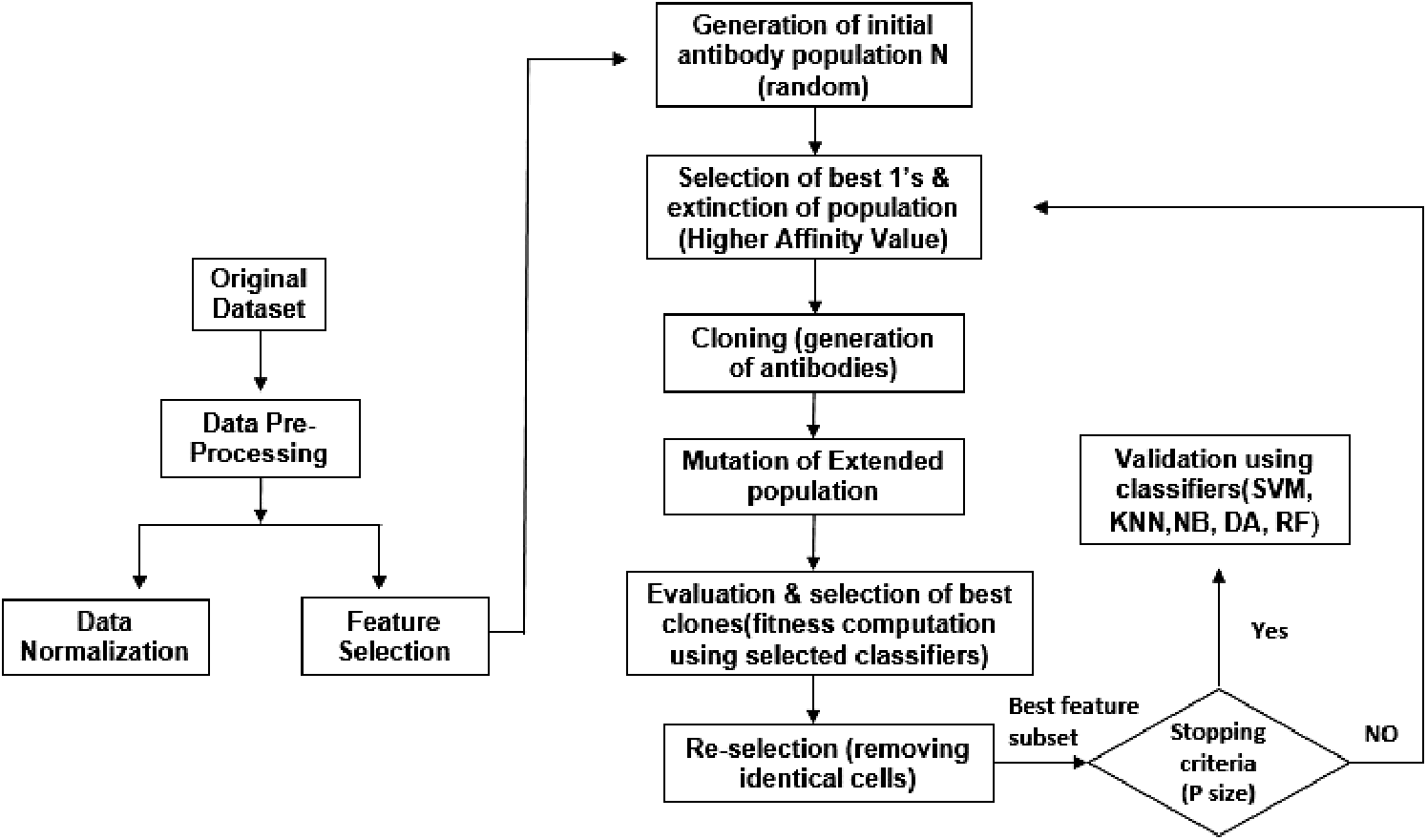
Figure 3: Our proposed approach
Step 1: Initialization: A random population is initialized. The number of generations is set as 5, 10, 20, 50 and 100 for all data sets.
Step 2: Main Loop: After the random initializing of the population, the cells undergo a clonal selection until a stopping condition is satisfied. Here, we set a stopping criterion of 50 for all data sets, which is the maximum number of iterations.
Step 3: Selection: To select the cells to be cloned, the Best Fitness Average is calculated. All the cells with an affinity higher than Best Fitness Average are selected and the remaining cells are then removed.
Step 4: Cloning: The clones generated are exactly proportional to the cell’s fitness value for which a clone is generated. Here the value of controlled parameter is Nc, i.e., the number of clones. The formula is given below:
Step 5. Mutation: All clones then undergo a somatic mutation so that they become variants of their parents. Each clone is mutated in inverse proportion to its fitness. The formula is given below:
where C’ is a mutated cell, c is the original cell, N(0,1) is a Gaussian random number of zero mean and standard deviation σ = 1, β is a control parameter which adjusts the mutation range and controls the decay of the inverse exponential function and value for β = 100 (user-specified value), α is the affinity proportional and f is the fitness of parent cell and f* is the fitness of an individual Ag or Ab in the population normalized in the interval [0.1].
Step 6: Re-Selection: performed on the basis of fitness function, i.e., the highest average accuracy.
Step 7: Suppression: The affinity of each cell in the network is determined. The suppression threshold is a controlled parameter whose value is set at 0.1 for our study. Suppress all cells except those having the highest fitness and affinities less than the suppression threshold. Then determine the number of network cells, named memory cells, after suppression.
Step 8: Diversity: At the end of each iteration, the newly-produced cells are added to the population; this is the same number of cells as those removed at the selection stage.
The experiment was performed on the Intel(R) Core (TM) processor with an 8 GB RAM installed on it using the Mat lab (R2018a) software tool.
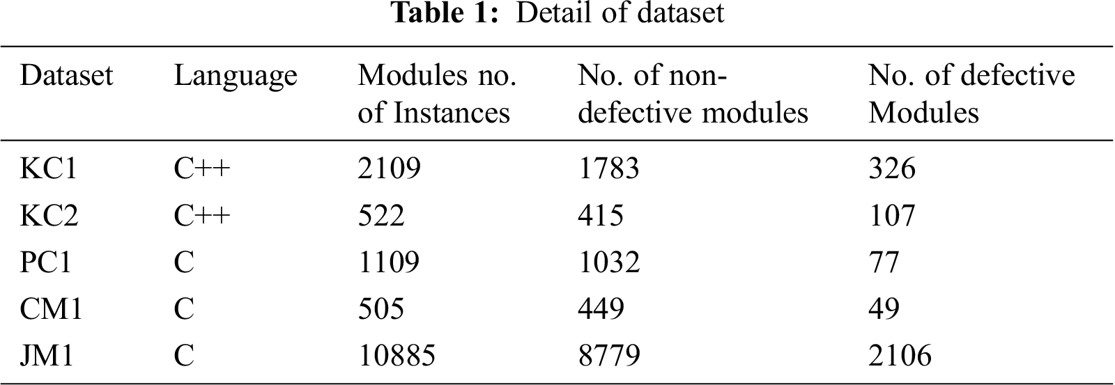
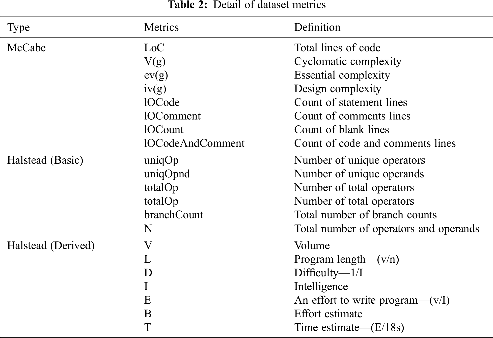
The NASA open-source MDP data sets are the ones most commonly used for SDP problems [27]. Five of the most used data sets, namely, KC1, KC2, CM1, PC1, and JM1, are used in this research. Each data set uses several quality metrics as input, and the data sets were developed by C/C++ language. NASA data sets have 22 method-level metrics from McCabe [37] and both basic and derived Halstead [37]. Tab. 1 presents the details of the data sets used in this study. Details of the metrics used for these data sets are presented in Tab. 2.
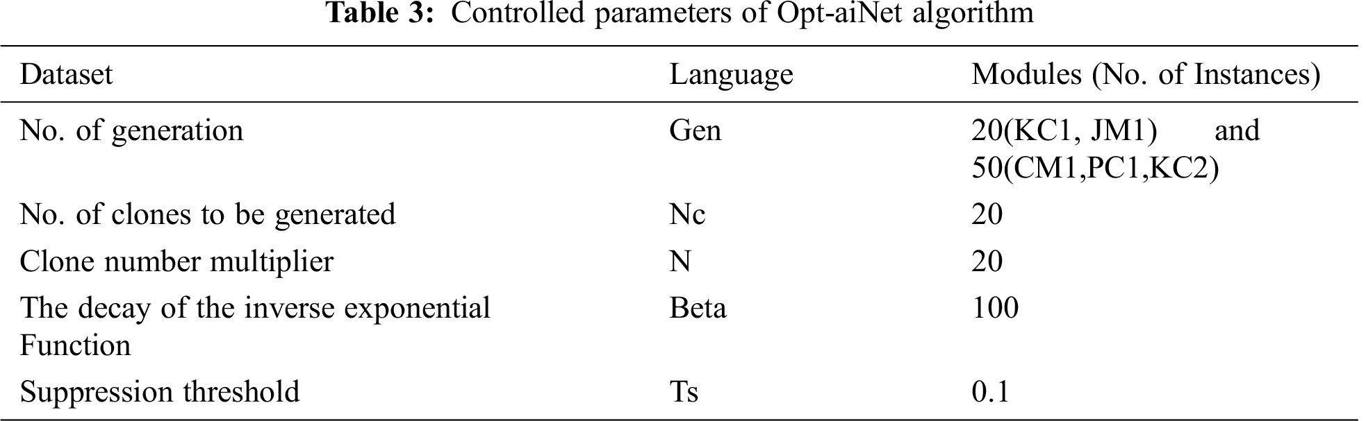
In this section, we report the results relevant to the impact of the Opt-aiNet-based FS technique on the accuracy of defect prediction. We conducted experiments with SDP datasets to classify data as either defective or not defective. We applied the Opt-aiNet-based feature subset selection techniques to the data sets. As stated earlier, Opt-aiNet computes all potential candidate solutions on the basis of their optimized fitness function and returns the best possible feature subsets. The controlled parameters of the Opt-aiNet algorithm for all five data sets are given in Tab. 3. The parameter values used in the study were based on the studies found in our literature review [6,27,38] except for the Gen value which depends on the size of the dataset used.
The selected features were fed to the six classifiers, SVM, KNN, NB, DT, LDA and RF on selected data subsets. In order to see whether the reduced feature subset would have an impact on predictive classification models, we applied six classifiers to the full data sets and used their results as a baseline. We used the 10-fold cross validation technology to avoid overfitting. In this study, confusion and accuracy were used for performance analysis by some of the most common measurement metrics AUC. Here we present the results of each of our experiments separately, to show that our proposed approach is an effective way to improve the accuracy of performance.
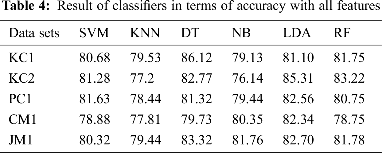
Datasets KC1, KC2, PC1, CM1 and JM1 from the PROMISE repository were used for experimentation. The data set KC1 contains a total of 2109 instances, KC2 contains 1109 instances, PC1 contains 522 instances, CM1 contains 505 instances and JM1 contains 10,885 instances. Tab. 4 presents the results of all six classifiers, i.e., SVM, KNN, DT, NB, LDA and RF in terms of accuracy with all features selected.
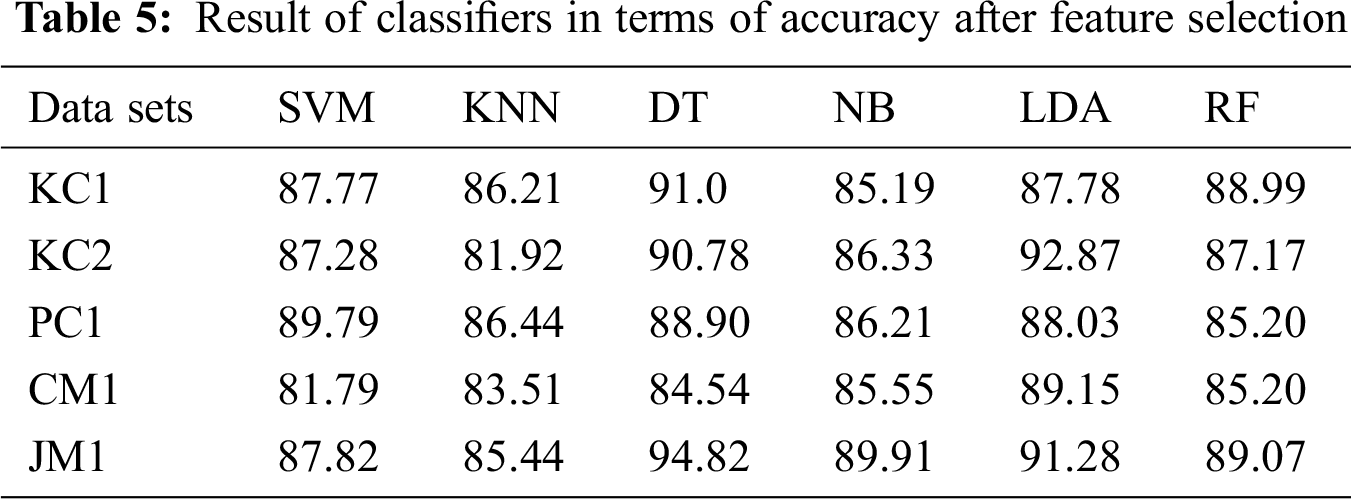
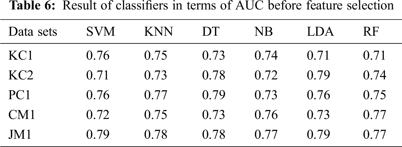
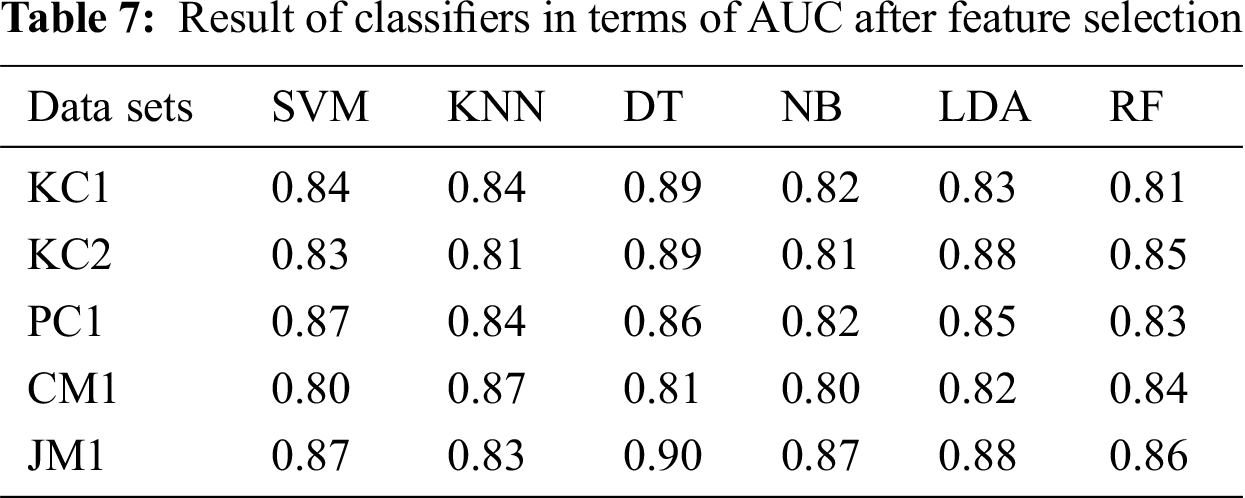
The results from the proposed approach to feature selection are presented in Tab. 5. The results show that the application of Opt-aiNet for FS significantly improves classifiers’ performance. There was a performance boost of up to 40% for the KC1 data set, 30% for the KC2 data set, 40% for the PC1 data set, 20% for the CM1 data set and 40% for the JM1 data set. DT provides the highest accuracy (94.82%) for the JM1 dataset with feature selection using Opt-aiNet. The results in Tabs. 6 and 7 in terms of AUC also reveal that feature selection significantly improves the bug prediction performance of the classifiers. Overall, DT shows the highest AUC Performance, namely, 0.90 for a JM1 data set with feature selection using Opt-aiNet.
7 A Comparison of the Proposed Approach (Opt-aiNet) with Other Techniques
7.1 A Comparison with Benchmark Techniques
We compared the performance of our proposed technique with the other state-of-the-art techniques reported in the literature. Most of the studies selected for comparison conducted experiments using the same five data sets (KC1, KC2, CM1, PC1 and JM1) as those used in our study, except for the study of R. Jayanthi and Lilly Florence and that of Afzal et al. [39]. Both of these studies used a different set of data sets with some being common to our study, i.e., KC1 and JM1 (R. Jayanthi and Lilly Florence) and CM1 (W. Afzal and R. Torkar), which we included here. We also compared our results with the latest techniques, such as CNN and DBN from studies by Hasanpour et al. [40] and Qasem et al. [41]. Another reason for selecting these studies was their higher number of citations, as well as the availability of their results in terms of AUC. The comparison Tab. 8 shows that the proposed approach results in an improved performance in terms of AUC for all the classifiers for the given data sets. The overall graphical representation of the comparison between the state-of-the-art techniques found in the literature with the proposed approach, i.e., using Opt-aiNet, is presented in Figs. 4–6 below.
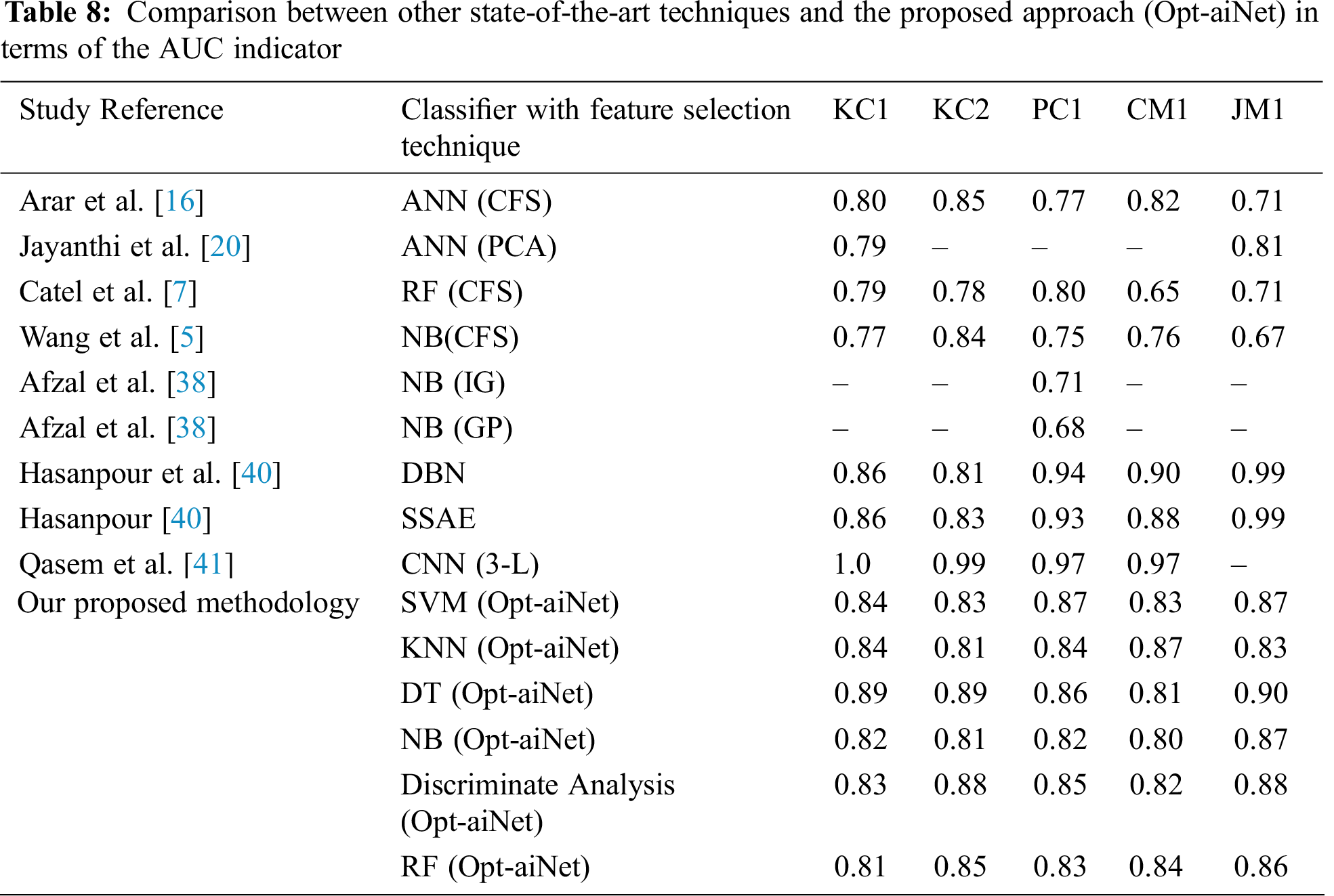
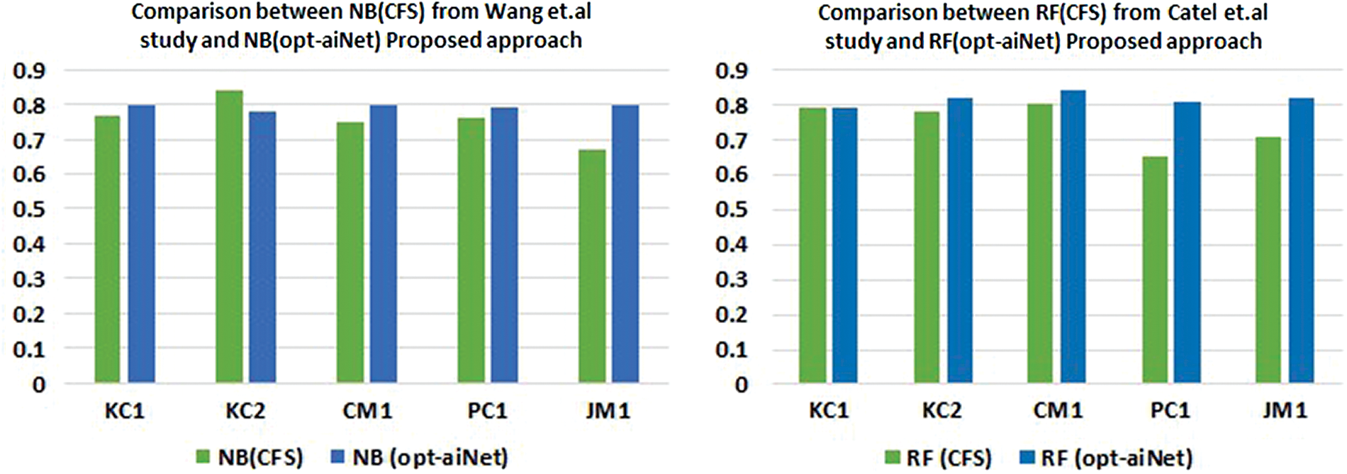
Figure 4: A graphical representation of the comparison between other state-of-the-art techniques and the proposed approach (Opt-aiNet) in terms of the AUC indicator
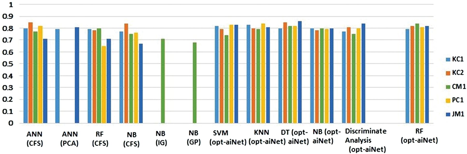
Figure 5: A graphical representation of a comparison between NB (CFS) from Wang et al.’s Study and RF (CFS) from Catel et al. and the proposed approach with FS with (Opt-aiNet)
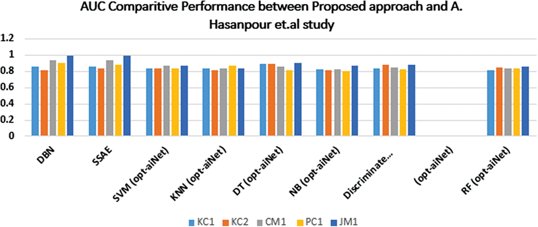
Figure 6: A graphical representation of a comparison between the proposed approach and Hasanpour et al.’s study
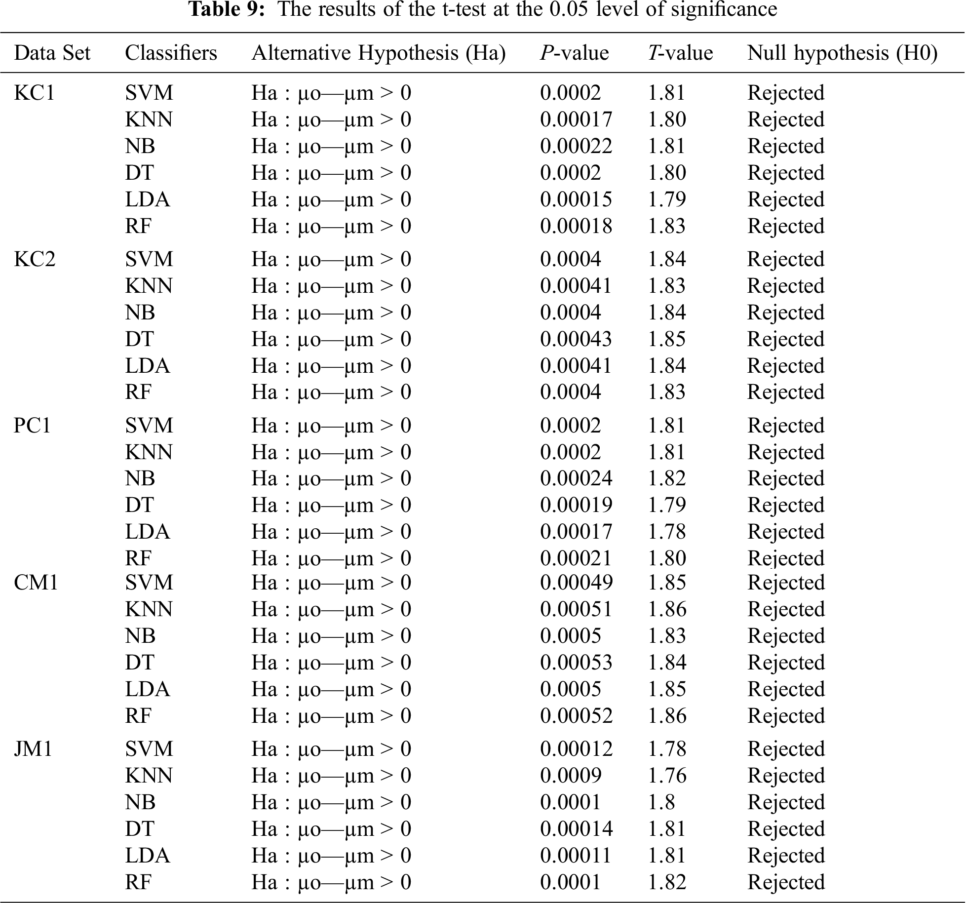
7.2 A Statistical Analysis of Opt-aiNet as FS
A t-test was performed using a 0.05 level of significance to compare the performance of our proposed technique. Let µm and µo be the mean performance accuracies from the application of the machine-learning classifiers with and without using Opt-aiNet, respectively. We tested the null hypothesis (H0: the Opt-aiNet in-conjunction with machine-learning classifiers does not make any difference in the classification performance in any case) against the alternate hypothesis (Ha: the Opt-aiNet in-conjunction with machine-learning classifiers increase the classification performance in any case). The t-test results given in Tab. 9 attest the significance of the Opt-aiNet because the Opt-aiNet in conjunction with the machine-learning classifiers, generated better results compared to the default machine-learning classifiers.
Early detection and prediction of software defects have a significant effect on software quality measurement. A software quality prediction model relies on the information mined from software measurement data and thus the better the selection of software metrics is by eliminating the redundant and less important features before training any defect prediction model the more probable it is to provide a more accurate end result. In this particular study, we examined the consequences of the FS technique on the overall performance accuracy of SDP. We introduced an Opt-aiNet based on the classification approach, which is a blend of an Opt-aiNet algorithm for feature selection and machine learning classifiers for data classification. When this proposed approach was used, the experimental results demonstrated a better performance. The results also showed that the selection technique of the DT classifier with Opt-aiNet features outperformed all other classifiers. It significantly improved prediction accuracy for all projects, with the most improved accuracy being 94.82% for the JM1 data set and the least improved accuracy being 84.55% for the CM1 data set. For future research, we intend to extend our work by optimizing the deep learning paradigms using our proposed feature selection technique to find out their impact on performance evaluation. Furthermore, the proposed approach may also be applied for improving decision support systems in other fields. We also intend to work on the issue of class imbalance and hyper-parameter optimization in the near future.
Funding Statement: The authors received no specific funding for this study.
Conflict of Interest: The authors declare that they have no conflicts of interest to report regarding the present study.
1. “IEEE standard glossary of software engineering terminology”, in IEEE Std 610.12-1990, pp. 1–84, 1990. [Google Scholar]
2. Malcolm Isaacs, World Quality Report, 2020. [Online]. Available: https://www.capgemini.com/service. [Google Scholar]
3. H. Wang, T. Khoshgoftaar and N. Seliya, “How many software metrics should be selected for defect prediction?,” in FLAIRS Conf., Palm Beach, Florida, USA, 2011. [Google Scholar]
4. H. Tanwar and M. Kakkar, “A review of software defect prediction models,” in Data management, analytics and innovation. Advances in intelligent systems and computing, V. Balas, N. Sharma, A. Chakrabarti, (eds.vol. 808. Springer, Singapore, pp. 89–97, 2019. [Google Scholar]
5. H. Wang, T. Khoshgoftaar and J. Van Hulse, “A comparative study of threshold-based feature selection techniques,” in 2010 IEEE Int. Conf. on Granular Computing, San Jose, CA, USA, pp. 499–504, 2010. [Google Scholar]
6. L. N. de Castro and J. Timmis, “An artificial immune network for multimodal function optimization,” in Proc. of the Congress on Evolutionary Computation, Honolulu, HI, USA, vol. 1, pp. 699–704, 2002. [Google Scholar]
7. C. Catal and B. Diri, “Investigating the effect of dataset size, metrics sets, and feature selection techniques on software fault prediction problem,” Information Sciences, vol. 179, no. 8, pp. 1040–1058, 2009. [Google Scholar]
8. C. Tantithamthavorn, S. McIntosh, A. Hassan and K. Matsumoto, “Automated parameter optimization of classification techniques for defect prediction models,” in Proc. of the 38th Int. Conf. on Software Engineering, Austin, TX, USA, pp. 321–332, 2016. [Google Scholar]
9. L. de Casto and F. J. Von Zuben, “An evolutionary immune network for data clustering,” in Proc. Sixth Brazilian Sym. on Neural Networks. Vol. 1. Riode Janeiro, Brazil, pp. 84–89, 2000. [Google Scholar]
10. J. Morera, C. Herrera, J. Arroyo and R. Fernandez, “An automated defect prediction framework using genetic algorithms: A validation of empirical studies,” Inteligencia Artificial, vol. 19, no. 57, pp. 114–137, 2016. [Google Scholar]
11. R. S. Wahon, “A systematic literature review of software defect prediction: Research trends, datasets, methods and frameworks,” Journal of Software Engineering, vol. 1, no. 1, pp. 1–16, 2015. [Google Scholar]
12. M. D’Ambros, M. Lanza and R. Robbes, “An extensive comparison of bug prediction approaches,” in Proc. 7th IEEE Work. Conf. Mining Software Repositories (MSRCape Town, South Africa, pp. 31–41, 2010. [Google Scholar]
13. Z. Chen, B. Boehm, T. Menzies and D. Port, “Finding the right data for software cost modeling,” IEEE Software, vol. 22, no. 6, pp. 38–46, 2005. [Google Scholar]
14. T. M. Khoshgoftaar, L. A. Bullard and K. Gao, “Attribute selection using rough sets in software quality classification,” International Journal of Reliability Quality and Safety Engineering, vol. 16, no. 1, pp. 73–89, 2009. [Google Scholar]
15. K. Gao, T. M. Khoshgoftaar, H. Wang and N. Seliya, “Choosing software metrics for defect prediction: An investigation on feature selection techniques,” Software: Practice and Experience, vol. 41, no. 5, pp. 579–606, 2011. [Google Scholar]
16. Ö.F. Arar and K. Ayan, “Software defect prediction using cost sensitive neural network,” Applied Soft Computing, vol. 33, no. 1, pp. 263–277, 2015. [Google Scholar]
17. Z. Xu, J. Liu, Z. Yang, G. An and X. Jia, “The impact of feature selection on defect prediction performance: An empirical comparison,” in 2016 IEEE 27th Int. Sym. on Software Reliability Engineering (ISSREOttawa, ON, Canada, pp. 309–320, 2016. [Google Scholar]
18. S. Wang, L. Taiyue and L. Tan, “Automatically learning semantic features for defect prediction,” in 2016 IEEE/ACM 38th Int. Conf. on Software Engineering (ICSEAustin, TX, USA, pp. 297–308, 2016. [Google Scholar]
19. J. Li, P. He, J. Zhu and M. R. Lyu, “Software defect prediction via convolutional neural network,” in IEEE Int. Conf. on Software Quality, Reliability and Security, Prague, Czech Republic, pp. 318–328, 2017. [Google Scholar]
20. R. Jayanthi and L. Florence, “Software defect prediction techniques using metrics based on neural network classifier,” Cluster Computing, vol. 22, no. S1, pp. 77–88, 2018. [Google Scholar]
21. C. Manjula and L. Florence, “Deep neural network-based hybrid approach for software defect prediction using software metrics,” Cluster Computing, vol. 22, pp. 9847–9863, 2018. [Google Scholar]
22. Z. Xu, J. Liu, X. Luo, Z. Yang, Y. Zhang et al., “Software defect prediction based on kernel PCA and weighted extreme learning machine,” Information and Software Technology, vol. 106, pp. 182–200, 2019. [Google Scholar]
23. X. Cai, Y. Niu, S. Geng, J. Zhang, Z. Cui et al., “An under-sampled software defect prediction method based on hybrid multi objective cuckoo search,” Concurrency and Computation: Practice and Experience, vol. 32, no. 5, pp. 1, 2020. [Google Scholar]
24. S. Kanwal, A. Hussain and K. Huang, “Novel artificial immune networks-based optimization of shallow machine learning (ML) classifiers,” Expert Systems with Applications, vol. 165, no. 1, pp. 113834, 2021. [Google Scholar]
25. F. O. de Franca, F. J. V. Zuben and L. N. de Castro, “An artificial immune network for multimodal function optimization on dynamic environments,” in Proc. of the 7th Annual Conf. on Genetic and Evolutionary Computation, Washington DC, USA, pp. 289–296, 2005. [Google Scholar]
26. F. Khan, S. Kanwal, S. Alamri and B. Mumtaz, “Hyper-parameter optimization of classifiers, using an artificial immune network and its application to software bug prediction,” IEEE Access, vol. 8, pp. 20954–20964, 2020. [Google Scholar]
27. D. Q. Vu, V. T. Nguyen and X. H. Hoang, “An improved artificial immune network for solving construction site layout optimization,” in 2016 IEEE RIVF Int. Conf. on Computing & Communication Technologies, Research, Innovation, and Vision for the Future (RIVFHanoi, Vietnam, pp. 37–42, 2016. [Google Scholar]
28. T. Cover and P. E. Hart, “Nearest neighbor pattern classification,” IEEE Transactions on Information Theory, vol. 13, no. 1, pp. 21–27, 1967. [Google Scholar]
29. S. K. Wajid, A. Hussain and K. Huang, “Three-dimensional local energy-based shape histogram (3d-leshA novel feature extraction technique,” Expert Systems with Applications, vol. 112, no. 4, pp. 388–400, 2018. [Google Scholar]
30. S. K. Wajid and A. Hussain, “Local energy-based shape histogram feature extraction technique for breast cancer diagnosis,” Expert Systems with Applications, vol. 42, no. 20, pp. 6990–6999, 2015. [Google Scholar]
31. T. Cover and P. E. Hart, “Nearest neighbor pattern classification,” IEEE Transactions on Information Theory, vol. 13, no. 1, pp. 21–27, 1967. [Google Scholar]
32. H. Zhang, “The optimality of Naive Bayes,” in FLAIRS2004 Conf., Miami Beach, Florida, USA, 2004. [Google Scholar]
33. X. Wu, V. Kumar, J. R. Quinlan, J. Ghosh, Yang Q. et al., “Top 10 algorithms in data mining,” Knowledge and Information Systems, vol. 14, no. 1, pp. 1–37, 2008. [Google Scholar]
34. G. J. McLachlan, Discriminant analysis and statistical pattern recognition. Wiley Interscience, Hoboken, NJ, USA, 2004. [Google Scholar]
35. T. K. Ho, “Random decision forests,” in Proc. of the 3rd Int. Conf. on Document Analysis and Recognition, Montreal, QC, pp. 278–282, 1995. [Google Scholar]
36. I. A. Basheer and M. Hajmeer, “Artificial neural networks: fundamentals, computing, design, and application,” Journal of Microbiological Methods, vol. 43, no. 1, pp. 3–31, 2000. [Google Scholar]
37. A Medium Corporation-ODSC Open data Science, 2018. https://medium.com/@ODSC/5-essential-neural-network-algorithm. [Google Scholar]
38. L. C. T. de Gomes, J. S. de Sousa, G. B. Bezerra, L. N. de Castro and F. J. V. Zuben, “Copt-aiNet and the gene ordering problem,” in Proc. of the Brazilian Workshop on Bioinformatics, Maca, RJ, Brazil, pp. 27–33, 2003. [Google Scholar]
39. W. Afzal and R. Torkar, “Towards benchmarking feature subset selection methods for software fault prediction,” in Computational Intelligence and Quantitative Software Engineering, Studies in Computational Intelligence. Vol. 617, 2016. [Google Scholar]
40. A. Hasanpour, P. Farzi, A. Tehrani and R. Akbari, “Software defect prediction based on deep learning models: Performance study,” arXiv: 2004.02589 [cs.SE], 2020. [Google Scholar]
41. O. A. Qasem and M. Akour, “Software Fault Prediction Using Deep learning algorithms,” International Journal of Open Source Software and Process, vol. 10, pp. 1–19, 2019. [Google Scholar]
 | This work is licensed under a Creative Commons Attribution 4.0 International License, which permits unrestricted use, distribution, and reproduction in any medium, provided the original work is properly cited. |