Intelligent Automation & Soft Computing DOI:10.32604/iasc.2021.016818
Article

An Adversarial Network-based Multi-model Black-box Attack

Bin Lin1, Jixin Chen2, Zhihong Zhang3, Yanlin Lai2, Xinlong Wu2, Lulu Tian4 and Wangchi Cheng5,*

1Sichuan Normal University, Chengdu, 610066, China
2School of Computer Science, Southwest Petroleum University, Chengdu, 610500, China
3AECC Sichuan Gas Turbine Establishment, Mianyang, 621700, China
4Brunel University London, Uxbridge, Middlesex, UB83PH, United Kingdom
5Institute of Logistics Science and Technology, Beijing, 100166, China
*Corresponding Author: Wangchi Cheng, Email: chengwc_szph@163.com
Received: 12 January 2021; Accepted: 27 April 2021

Abstract: Researches have shown that Deep neural networks (DNNs) are vulnerable to adversarial examples. In this paper, we propose a generative model to explore how to produce adversarial examples that can deceive multiple deep learning models simultaneously. Unlike most of popular adversarial attack algorithms, the one proposed in this paper is based on the Generative Adversarial Networks (GAN). It can quickly produce adversarial examples and perform black-box attacks on multi-model. To enhance the transferability of the samples generated by our approach, we use multiple neural networks in the training process. Experimental results on MNIST showed that our method can efficiently generate adversarial examples. Moreover, it can successfully attack various classes of deep neural networks at the same time, such as fully connected neural networks (FCNN), convolutional neural networks (CNN) and recurrent neural networks (RNN). We performed a black-box attack on VGG16 and the experimental results showed that when the test data classes are ten (0–9), the attack success rate is 97.68%, and when the test data classes are seven (0–6), the attack success rate is up to 98.25%.

Keywords: Black-box attack; adversarial examples; GAN; multi-model; deep neural networks

1  Introduction

Deep neural networks have achieved great success in various computer vision tasks, such as image recognition [1,2], object detection [3] and semantic segmentation [4], etc. However, recent research has shown that deep neural networks are vulnerable to adversarial examples [5], a modification of the clean image by adding well-designed perturbations in a way that the changes are imperceptible to the human eye. Since adversarial examples were introduced, adversarial has attacks have attracted a lot of attention [6,7]. Most of current attack algorithms are gradient-based white-box attacks [8] which have the complete knowledge of the targeted model including its parameter values, architecture and calculate the gradient of the model to generate the adversarial examples with neural networks, but these adversarial examples have poor transferability and can attack specific deep learning models only. In fact, it is undeniable that in some instances, the adversary has a limited knowledge of the model, which in turn leads to unsuccessful attacks. Therefore, it is of great importance to study black-box attacks which can make up for the deficiency of the white box attacks.

Fig. 1 shows clean images in the front row and their corresponding adversarial images in the bottom row. These adversarial images are still recognizable to the human eye, but can fool the deep learning models. Since white-box attacks have their deficiency mentioned above, to address this issue, we propose a black-box attack algorithm to produce adversarial examples that can fool DNNs even with limited knowledge of the model by using multiple classification (MC) models and distilling useful models to train the generator and discriminator.

Figure 1: Comparison of clean images and adversarial images

2  Related Work

2.1 Adversarial Examples

Adversarial examples were introduced in 2013 by Szegedy et al. and their researches have demonstrated that deep neural networks, CNNs included are vulnerable to adversarial examples. Meanwhile, there are many other researches dedicated to adversarial attacks. The majority of them are based on optimization by minimizing the distance between the adversarial images and the clean images so as to cause the model to make wrong classification prediction. Some attack strategies require access to the gradients or parameters of the model, yet these strategies are limited to gradient-based models only. (e.g., neural networks). Others only need have access to the output of the model.

Fig. 2 is the generation process of adversarial examples. The attack algorithm firstly computes the perturbations by calling the deep learning model and then creates the adversarial examples by adding the perturbations to the clean images to fool the model.

Figure 2: Generating adversarial example

2.2 Attack Methods

There are two common types of adversarial attacks: white-box attacks and black-box attacks. The adversarial attacks are called white-box attacks when the complete information of the targeted model is fully known to the adversary. Alternatively, when the adversary has limited knowledge of the targeted model and creates adversarial examples by having access to the input and output of the model, they are called black-box attacks. Among the existing attacks, the white-box attack algorithm predominates.

2.2.1 White-box Attacks

In white-box attacks, L-BFGS [9] is one of white-box attacks to generate adversarial examples for deep learning model. However, there are imperfections in this attack algorithm. For example, it is very slow to generate the adversarial examples and these examples can be well-defended by reducing their quality. Goodfellow et al. [10] proposed Fast Gradient Sign Method (FGSM), which generates adversarial examples by incrementing the gradient direction of the model loss. Due to the high computational cost of L-BFGS and the low attack success rate of FGSM, the Basic Iterative Method, also called I-FGSM, was proposed by Kurakin et al. [11]. BIM can reduce the computational costs with iterative optimization and increase the attack success rate, so highly-aggressive adversarial examples can be created after a small number of iterations. Projected Gradient Descend (PGD) in Madry et al. [12] which can produce adversarial examples via randomly initializing the search in a certain azimuth class of the clean images and then iterating several times and as a result, it became the most powerful first-order adversarial attack. That is, if the defense method can successfully defend the attack of PGD algorithm, then it can defend other first-order attack algorithms as well. Carlini et al. [13] attack (C&W) designed a loss function and a search for adversarial examples by minimizing the loss function and they applied Adam [14], which projects the results onto box constraints at each step to achieve the strongest L2 attack, so as to solve the optimization problem and handled box constraints.

2.2.2 Black-box Attacks

Black-box attacks have two categories: those with probing and those without probing. As for the former, the adversary knows little or nothing about the model but can have access to the model’s output through the input, while the latter implies that the adversary has limited knowledge of the model. Some studies [15,16] pointed out that adversarial examples generated by black-box attacks can fool more than one model.

2.3 Generative Adversarial Networks

The generative adversarial networks proposed by Goodfellow et al. [17] is an unsupervised learning algorithm inspired by the two-person zero-sum games in game theory. Its unique adversarial training idea can generate high quality examples, so it has more powerful feature learning and representation capabilities than traditional machine learning algorithms. GAN consists of a generator and a discriminator, each of which updates its own parameters to minimize the loss during the training process of the model, and finally reaches a Nash equilibrium state through continuous iterative optimization. However, there is no way to control the model because the process is too free in generating lager images. To overcome the limitations of GAN, Conditional GAN (CGAN) was proposed by Mirza et al. [18] and they added constraints to the original GAN to direct the sample generation process. After that, many advancements in designing and training GAN models have been made, most significantly the Deep Convolutional GAN (DCGAN) proposed by Radford et al. [19], which is a combination of CNN and GAN and has substantially improved the quality and diversity of the generated images. Fig. 3 is a schematic diagram of the structure of GAN.

Figure 3: Generative adversarial networks [17]

3  Methodology

3.1 Problem Definition

Suppose I is a clean image, Ia is an adversarial image, G is a generator, D is a discriminator, and CMA,CMB,CMC,CMD are four classification models, where CMA is a CNN, CMB is a FCNN, CMC is a RNN, and CMD is a CNN with a more complex structure. We choose CMA as a local model and distill model [20] CMD′ from CMD . We expect to train the generator and discriminator by calling CMA,CMB,CMC and CMD′ . As a result, the adversarial examples generated by this trained model are able to attack CMD with a high attack success rate (ASR). I and Ia can be expressed by the following equation:

Ia=I+G(I) (1)

3.2 Network Architecture

The model proposed in the paper consists of a generator and a discriminator of GAN. The generator is similar to the way the encoding network in VAE [21], where examples are input to generate perturbations, and then these perturbations are added to the original input to get the adversarial examples. While the discriminator is a simply a classifier and it is used to distinguish the clean images from the adversarial images created by the generator. The model is shown in Fig. 4.

Figure 4: Structure of our method. The clean image I is passed into the generator to obtain G(I). CMA,CMB,CMC and CMD are four classification models which are FCNN, CNN, LSTM and VGG16 [22]. CMD′ is the distillation model of CMD . G(I) is input into the four classification models in the figure, and the output of the model (probability) and the generator loss can be obtained. Then G(I) is input into the discriminator and discriminator loss can be calculated

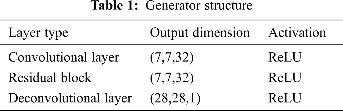
Tab. 1 is the structure of the generator.

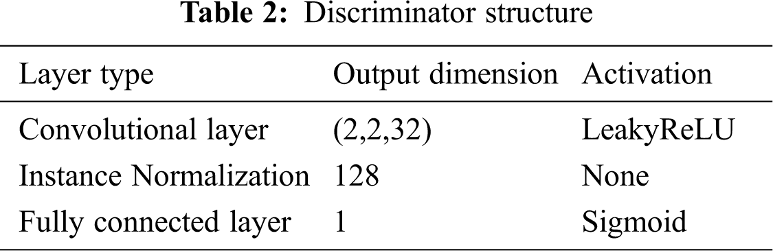
The network architecture of discriminator is similar to that in DCGAN. The clean and generated images are respectively fed into the discriminator and then passes three convolutional layers, one fully connected layer and a sigmoid activation function. The discriminator D is to make the prediction of the clean images as close to 1 as possible and the generated images approximate 0. The network architecture of discriminator is presented in Tab. 2.

3.3 The Algorithm for Generating Adversarial Examples

The algorithm for generating adversarial examples is as follows. The inputs are clean image I and four pre-trained models, the output is the adversarial images. The whole process starts with obtaining the distillation model CMD′ and then the model is trained according to Eqs. (2) and (5) to minimize the loss so that the model output the adversarial images successfully.

3.4 Loss Function

The loss function of the generative model contains that of the discriminator and generator. The loss function of the discriminator can be described as follows:

LD=Lfake+Lreal (2)

To make the discriminator converge, we choose the mean square error (MSE) [23] as the loss function of the discriminator. From Eq. (2), it can be seen that the loss function is made up of the real and the fake loss. Where the real loss can be described as:

Lreal=MSE(D(I),1) (3)

I refers to the clean image, and D(I) is the output. Since training the discriminator is to make the clean image approach to 1, D(I) is combined with the all-1 vector to compute the MSE. Meanwhile, we expect the generated image to become near 0, so the generated examples loss can be expressed as follows:

Lfake=MSE(D(G(I))+I,0) (4)

The loss function of the generator consists of three parts, as shown in Eq. (5), on the premise of α=β=γ=1 , the generated adversarial examples are best.

LG=αLg+βLperturb+γLadv (5)

The first part is to make the generated image as close to the real image, so the first part is MSE, as shown in Eq. (6).

Lg=MSE(G(I)+I,1) (6)

The goal of the second part is making the output G(I) of the generator as close as to 0, so we add the hinge loss to the L2 norm. ε is a hyperparameter used to stabilize the training of generator.

Lperturb=max(0,||G(I)||2−ε) (7)

The third part is to enable the generated examples to deceive the classification model, so the loss function can be defined by:

Ladv=f(C(G(I)+I),y) (8)

In Eq. (8), C represents the multiple models, including CMA,CMB,CMC and the distillation model CMD′ , f stands for the loss function and y symbolizes the one-hot vector transformed from the real label. As a result, its probability value can be obtained by adding the output of the generator and the clean image as the input of the multiple models, and then the loss can be calculated by using label y .

4  Experiment

4.1 Environment and Dataset

For the experimental environment, TensorFlow was applied as the deep learning framework, and the graphics card was NVIDIA GeForce GTX1080Ti. CUDA and cuDNN were configured for graphics card acceleration training.

The data set in the experiment was the MNIST handwritten digits data set, which consists of 60,000 train set images and 10,000 test set images. These images have been pre-processed with a uniform size of 28*28, which reduces the complex operations of data collection and pre-processing, and allow us to utilize them with only some normalization.

4.2 Threat Model

CMA is used as a local model to get the distillation model CMD′ from CMD , and our goal is training the generative model by calling the multi-model (excluding model CMD ). The generated adversarial examples can not only attack multi-model for auxiliary training but also the model CMD , i.e., VGG16.

4.3 Results and Analysis

White-box attacks are the most commonly used in adversarial attacks and they have their deficiency mentioned above. To prove that our method is effective, we generated 10,000 adversarial examples with an assumption of the test data set of MNIST, as shown in Fig. 5, and then classified them with CMA,CMB,CMC and CMD respectively. Tab. 3 shows the black-box attack algorithm proposed by Xiao et al. [24].

Figure 5: A comparison of clean images and adversarial images. The first two rows are clean images sampled from the MNIST data set, and the last two rows are their corresponding adversarial images produced by our method, which are able to force CMD to make wrong classification prediction with limited knowledge of the model CMD

CMA as a local model, CM′ as the distillation model get by CMA distilling CMB,CMC and CMD respectively. They are used as the target models for training the generative models. Accuracy is calculated on models CMA,CMB,CMC and CMD after obtaining the adversarial examples.

As we can see in Tab. 4, we have adopted multi-model to train the generative model, and the ASR of CMD has been improved for both static and dynamic distillation. We also experiment on MNIST with 7 classes (0–6) further improved by ASR, and the experimental results are shown in Tab. 5.

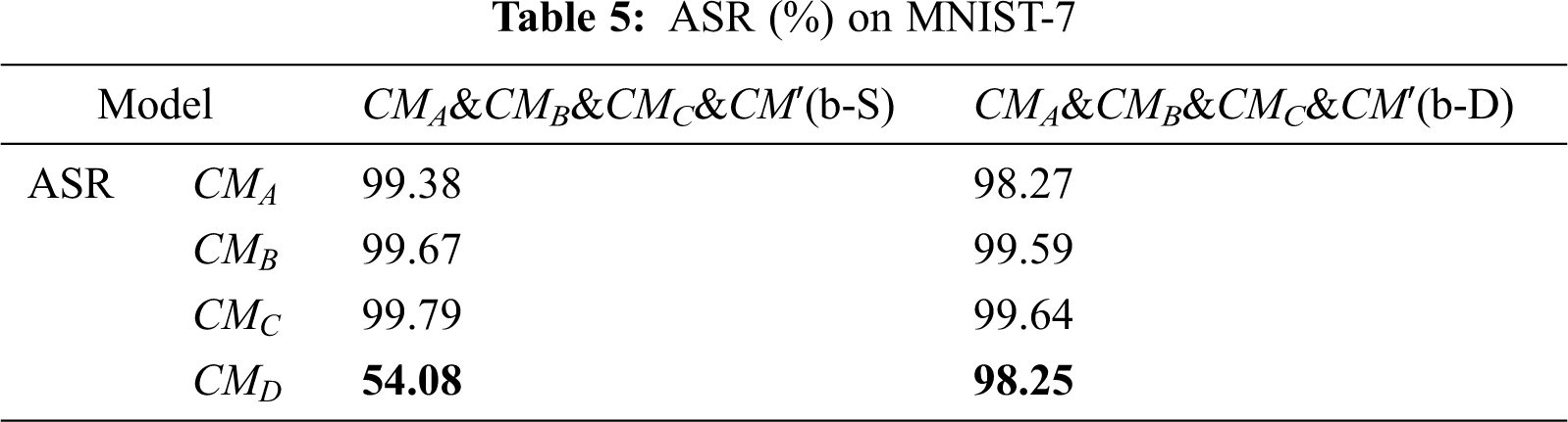
As shown in the table above, the ASR of VGG16 has increased from 97.39% to 98.25%, which proves that our method can effectively perform black-box attack on VGG16.

5  Conclusion

In this paper, we proposed a black-box attack algorithm based on the GAN network architecture. Compared with other adversarial attack algorithms, this method generates adversarial examples with better transferability and higher ASR for the model. We use various classes of neural networks to assist in the training of the model, and experiments conducted on MNIST have validated the effectiveness and efficiency of our method.

Funding Statement: This work was supported by Scientific Research Starting Project of SWPU [No. 0202002131604]; Major Science and Technology Project of Sichuan Province [No. 8ZDZX0143, 2019YFG0424]; Ministry of Education Collaborative Education Project of China [No. 952]; Fundamental Research Project [Nos. 549, 550].

Conflicts of Interest: The authors declare that they have no conflicts of interest to report regarding the present study.

References

 1.  D. Keysers, T. Deselaers, C. Gollan and H. Ney, “Deformation models for image recognition,” IEEE Transactions on Pattern Analysis and Machine Intelligence, vol. 29, no. 8, pp. 1422–1435, 2007. [Google Scholar]

 2.  K. Zhang, Y. Guo and X. Wang, “Multiple feature reweight densenet for image classification,” IEEE Access, vol. 7, pp. 9872–9880, 2019. [Google Scholar]

 3.  A. Qayyum, I. Ahmad, M. Iftikhar and M. Mazher, “Object detection and fuzzy-based classification using UAV data,” Intelligent Automation & Soft Computing, vol. 26, no. 4, pp. 693–702, 2020. [Google Scholar]

 4.  K. Akadas and S. Gangisetty, “3D semantic segmentation for large-scale scene understanding,” in Proc. ACCV, 2020. [Google Scholar]

 5.  C. Szegedy, W. Zaremba, I. Sutskever, J. Bruna, D. Erhan et al., “Intriguing properties of neural networks,” in Proc. ICLR, Banff, CAN, pp. 142–153, 2014. [Google Scholar]

 6.  Z. G. Qu, S. Y. Chen and X. J. Wang, “A secure controlled quantum image steganography algorithm,” Quantum Information Processing, vol. 19, no. 380, pp. 1–25, 2020. [Google Scholar]

 7.  X. Li, Q. Zhu, Y. Huang, Y. Hu, Q. Meng et al., “Research on the freezing phenomenon of quantum correlation by machine learning,” Computers Materials & Continua, vol. 65, no. 3, pp. 2143–2151, 2020. [Google Scholar]

 8.  S. Nidhra and J. Dondeti, “Black-box and white-box testing techniques-a literature review,” International Journal of Embedded Systems and Applications, vol. 2, no. 2, pp. 29–50, 2012. [Google Scholar]

 9.  C. D. Liu and J. Nocedal, “On the limited memory BFGS method for large scale optimization,” Mathematical Programming, vol. 45, no. 1, pp. 503–528, 1989. [Google Scholar]

10. I. J. Goodfellow, J. Shlens and C. Szegedy, “Explaining and harnessing adversarial examples,” in Proc. ICLR, California, CA, USA, pp. 226–234, 2015. [Google Scholar]

11. A. Kurakin, I. J. Goodfellow and S. Bengio, “Adversarial examples in the physical world,” in Proc. ICLR, Puerto Rico, USA, pp. 99–112, 2016. [Google Scholar]

12. A. Madry, A. Makelov, L. Schmidt, D. Tsipras and A. Vladu, “Towards deep learning models resistant to adversarial attacks,” in Proc. ICLR, Vancouver, Canada, pp. 542–554, 2018. [Google Scholar]

13. N. Carlini and D. Wagner, “Towards evaluating the robustness of neural networks,” in Proc. IEEE Sym. on Security and Privacy, pp. 39–57, 2017. [Google Scholar]

14. D. P. Kingma and J. L. Ba, “Adam: A method for stochastic optimization,” in Proc. ICLR, California, CA, USA, pp. 428–440, 2015. [Google Scholar]

15. X. Li, Q. Zhu, Q. Meng, C. You, M. Zhu et al., “Researching the link between the geometric and Rènyi discord for special canonical initial states based on neural network method,” Computers Materials & Continua, vol. 60, no. 3, pp. 1087–1095, 2019. [Google Scholar]

16. D. Zheng, Z. Ran, Z. Liu, L. Li, L. Tian et al., “An efficient bar code image recognition algorithm for sorting system,” Computers Materials & Continua, vol. 64, no. 3, pp. 1885–1895, 2020. [Google Scholar]

17. I. J. Goodfellow, J. Pouget-Abadie, M. Mirza, B. Xu, D. Warde-Farley et al., “Generative adversarial nets,” Proc. NIPS, vol. 27, pp. 2672–2680, 2014. [Google Scholar]

18. M. Mirza and S. Osindero, “Conditional generative adversarial nets,” arXiv preprint arXiv: 1411.1784, pp. 145–152, 2014. [Google Scholar]

19. A. Radford, L. Metz and S. Chintala, “Unsupervised representation learning with deep convolutional generative adversarial networks,” in Proc. ICLR, Puerto Rico, USA, pp. 300–312, 2016. [Google Scholar]

20. G. E. Hinton, O. Vinyals and J. Dean, “Distilling the knowledge in a neural network,” ArXiv Preprint ArXiv: 1503.02531, 2015. [Google Scholar]

21. D. P. Kingma and M. Welling, “Auto-encoding variational bayes,” in Proc. ICLR, Banff, Canada, pp. 244–255, 2014. [Google Scholar]

22. A. Sengupta, Y. Ye, R. Wang, C. Liu and K. Roy, “Going deeper in spiking neural networks: VGG and residual architectures,” Frontiers in Neuroscience, vol. 13, pp. 95, 2019. [Google Scholar]

23. L. Hu and P. M. Bentler, “Cutoff criteria for fit indexes in covariance structure analysis: Conventional criteria versus new alternatives,” Structural Equation Modeling, vol. 6, no. 1, pp. 1–55, 1999. [Google Scholar]

24. C. Xiao, B. Li, J. Y. Zhu, W. He, M. Liu et al., “Generating adversarial examples with adversarial networks,” in Proc. IJCAI, Stockholm, Sweden, pp. 3905–3911, 2018. [Google Scholar]

This work is licensed under a Creative Commons Attribution 4.0 International License, which permits unrestricted use, distribution, and reproduction in any medium, provided the original work is properly cited.