Intelligent Automation & Soft Computing DOI:10.32604/iasc.2021.020010
Article

Method of Bidirectional LSTM Modelling for the Atmospheric Temperature

Shuo Liang1, Dingcheng Wang1,*, Jingrong Wu1, Rui Wang1 and Ruiqi Wang2

1Nanjing University of Information Science and Technology, Nanjing, 230031, China
2Australian National University, Canberra, 2601, Australia
*Corresponding Author: Dingcheng Wang. Email: dcwang2005@126.com
Received: 05 May 2021; Accepted: 17 June 2021

Abstract: Atmospheric temperature forecast plays an important role in weather forecast and has a significant impact on human daily and economic life. However, due to the complexity and uncertainty of the atmospheric system, exploring advanced forecasting methods to improve the accuracy of meteorological prediction has always been a research topic for scientists. With the continuous improvement of computer performance and data acquisition technology, meteorological data has gained explosive growth, which creates the necessary hardware support conditions for more accurate weather forecast. The more accurate forecast results need advanced weather forecast methods suitable for hardware. Therefore, this paper proposes a deep learning model called BL-FC based on Bidirectional Long Short-Term Memory (Bi-LSTM) Network for temperature modeling and forecasting, which is suitable for big data processing. BL-FC consists of four layers: the first layer is a Bi-LSTM layer, which is used to learn features from continuous temperature data in forward and backward directions; the other three layers are fully connected layers, the second and third layers are used to further extract data features, and the last layer is used to map the final output of temperature prediction. Based on the meteorological data of 19822 consecutive hours provided by Belmalit Mayo Weather Station in Mayo County, Ireland, the data set is established by using the sliding window method. Compared with other three different deep learning models, including Long Short-Term Memory (LSTM), Gated Recurrent Unit (GRU), and Recurrent Neural Network (RNN), the BL-FC model has higher short-term temperature prediction accuracy, especially in the case of abnormal temperature.

Keywords: Atmospheric temperature; prediction; deep learning; Bi-LSTM

1  Introduction

The definition of temperature in meteorology is a physical quantity that expresses the degree of coldness and heat of the air. The statistics and prediction of temperature are essential in agriculture [1–3], industry [4], and human daily life [5–7]. In recent years, with population growth and accelerated urbanization, the greenhouse effect is consistently increasing [8], extremely, weather has become more and more frequent [9], heat and cold wave has caused serious threats to the normal production and life of human beings. Therefore, an accurate temperature prediction model is urgently needed.

Traditional meteorological predicting research mainly focuses on establishing temperature predicting models based on several specific meteorological factors. For example, Wang et al. [10], predict the interannual variation of temperature by studying atmospheric circulation and southern oscillation index. Brands et al. [11] uses traditional statistical methods, building a statistical downscaling model to predict the daily temperature of northwestern Spain. However, the temperature is affected by many factors including altitude, terrain, illumination, distance from the sea, few human factors [12]. Also, temperature is a sequential data that has a strong spatiotemporal. Traditional meteorological prediction methods only consider several specific factors, and always ignore the sequential data feature, which leads to large predict errors.

Meteorological data is typical sequential data. So, time series prediction methods have been used to deal with many weather factors prediction problems such as wind speed [13], temperature [14,15], and precipitation [16]. Temperature prediction is one of the most important tasks in meteorology, accurate temperature prediction is of great significance to the economy and human daily life. The Support Vector Machine (SVM) [14], and Back Propagation (BP) neural network [15] are the most commonly used temperature prediction methods. However, the above methods all have several defects in the process of temperature prediction. BP neural network ignores the sequential feature of temperature, SVM does not perform very well when the data set is large.

Deep learning network is suitable for big data learning by its iterative and deep structure. There are many sorts of deep learning, such as, RNN, GRU, and LSTM etc. RNN uses a loop structure to capture the feature of sequential data. The special loop structure can reserve information from a long context window. GRU and LSTM are improved versions of RNN, using a special gated structure to overcome the shortcomings of RNN. In recent years, with the development of computing power, modification of network architecture, LSTM, and its variants have made a big breakthrough in the prediction of time series and can handle a lot of tasks. For example, Chen et al. [17] uses LSTM network to predict the energy consumption in Beijing, Yan et al. [18] propose an improved method for the prediction of the number of covid-19 confirmed cases based on LSTM and Zhang et al. [19] come up with a novel Bi-LSTM and attention mechanism based neural network for answer selection in community question answering. Therefore, LSTM has been applied to modelling and predicting the water level in Yangtze River [20], and air temperature [21].

Although LSTM overcomes the defects of RNN, it only processes time series in forward direction. Temperature data fluctuates slowly over time, the temperature of a single time point is affected by both past and future temperatures. Therefore, this paper adopts a model based on Bi-LSTM to solve the problems above. The structure of Bi-LSTM ensures that it can process data in both forward and backward directions. The experiments were carried out on the data provided by the Mayo Weather Station. Four time-series prediction models are used to compare the model performance. The prediction results indicate the Bi-LSTM-Based model outperforms the other three models in every metric we adopted.

2  Methods and Materials

2.1 Experimental Dataset

The data used in this paper is the continuous 198112 hours of meteorological data provided by the Moyo Weather Station. We have selected 15 meteorological features as input data. They are latitude, longitude, precipitation amount, temperature, wet bulb temperature, dew point temperature, vapour pressure, relative humidity, mean sea level pressure, mean hourly wind speed, predominant hourly wind direction, sunshine duration, visibility, cloud ceiling height and cloud amount.

Data preprocessing is an essential step for deep learning models, proper data preprocessing can not only improve the accuracy of predictions, but also speed up the training process. Visibility, cloud ceiling height, and cloud amount have missing values. Therefore, we fill the missing values with the mean of visibility, cloud ceiling height, and cloud amount. Besides, different features are in different magnitudes, which will increase the difficulty of model training. In this paper, we use normalization to solve the problem. The formula of normalization is shown in Eq. (1).

xi=xiabs(xmax) (1)

xi represents the value of the element to be processed, xmax represents the maximum value of each column of raw data, through the normalization all data are mapped to [–1,1], which eliminates the huge gap between magnitudes of different meteorological features.

After the normalization, standardization is used to fit the data to a normal distribution, which can accelerate the speed of gradient descent during the backpropagation. The specific formula is shown in Eq. (2).

xi=xi−μσ (2)

Bi-LSTM is a variant of LSTM, so the input data needs to be time series. The data provided by Moyo Weather Station is discrete and cannot be directly inputted into the model. Here we adopt a sliding window method to transform the discrete data into time series. Two windows are used here, the first one is for sample data, and the second one is for target data. The length of the sliding windows can be adjusted as needed. Generally speaking, the longer the sample data is, the more accurate the predicted result is. In this paper, we uniformly use a 4:1 sample target ratio to construct datasets. The step length of the sliding window is set to 1, which means that after the sample set and result set are constructed, the window moves forward by one hour. It not only ensures the sufficiency of the dataset but also conforms to the continuous regularity of time series. The structure of two sliding window: sample data window S and target data window p are shown in Eqs. (3) and (4).

S=[[am1,am2,am3,……………,am15][am+11,am+12,am+13,…,am+115]...[a2m1,a2m2,a2m3,…………,a2m15]] (3)

p=[[t2m+1][t2m+2]...[t2m+n]] (4)

In Eq. (3), the matrix elements have the form of amj , represents the data of the j-th feature collected at the m-th moment, and in Eq. (4), the matrix elements have the form of t2m+i , represents the real temperature at the (2m + i)-th moment. These two matrices represent the use of m hours meteorological data to predict the temperature in the next n hours and m:n is the sample and target data radio. Therefore, after determining the sample target ratio, we can construct a new dataset as long as we keep moving the sliding window forward.

By using the sliding window method above, we can transform the raw data into different datasets according to different sample target ratios.

2.2 BL-FC: The Proposed Model for Temperature Prediction

The dataset provided by Moyo Weather Station contains 198112 consecutive hours of weather and temperature data. Two visualizations of the dataset are made based on the dataset. Fig. 1 describes the change of temperature in 3 years, and Fig. 2 shows the fluctuation trend of temperature in a month.

From Fig. 1 we can see that the long-term temperature change in the local area has a strong periodicity. The fluctuation of the temperature follows a fixed pattern, which provides a good realistic basis for the use of time series prediction models.

According to Fig. 2, the trend of short-term temperature is no longer periodic but fluctuates constantly and is accompanied by some abnormal temperatures. However, there is still a strong correlation between temperature data, the temperature at a specific moment is affected by adjacent temperatures in both forward and backward directions.

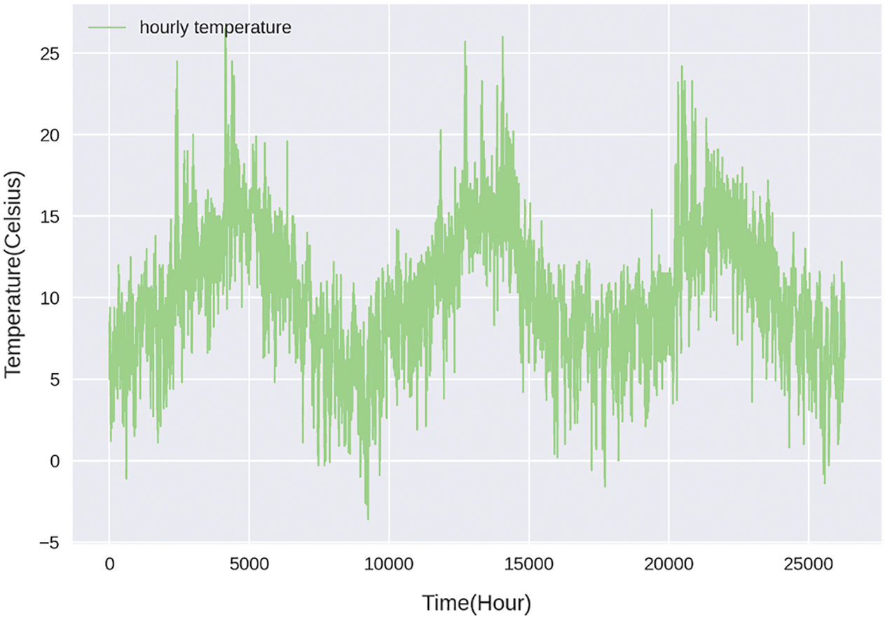
Figure 1: The changes of temperature in three years

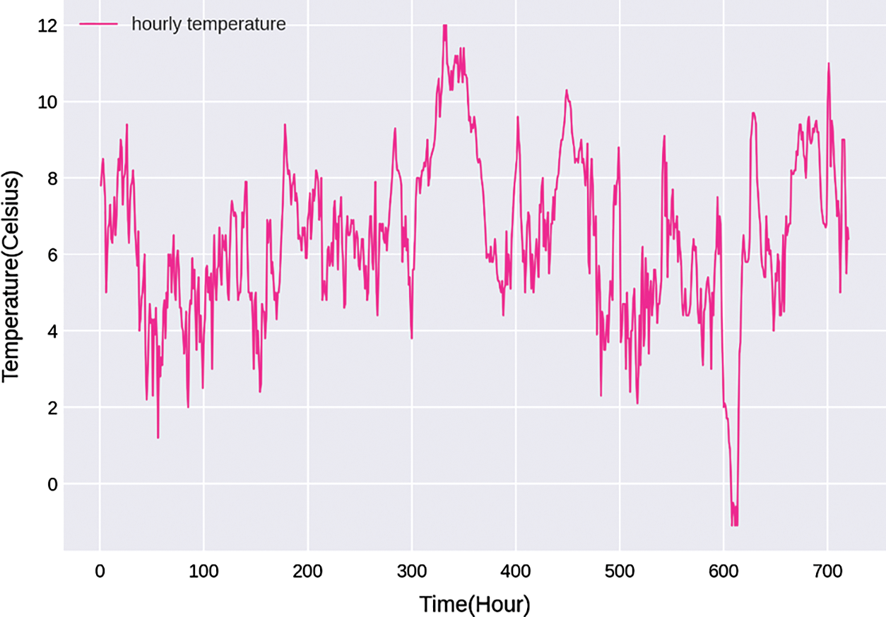
Figure 2: The changes of temperature in one month

In conformity with the previously analyzed temperature characteristics, we propose a short-term prediction model called BL-FC based on Bi-LSTM. Common LSTM-Based [22] models incorporate additional "gates" to learn features from a long sequence of input data, thus performing well in the prediction of time series. Compared with LSTM, Bi-LSTM enables additional training by traversing the input data twice [23] and can capture the information in forward and backward directions. So Bi-LSTM is utilized in the first module of BL-FC to extract features from fluctuating temperature. Then the output data of Bi-LSTM layer is conveyed to the fully connected layers in the second and the third module for further fitting and extracting operation. The last layer is also a fully connected layer, which is applied to map the output of the whole model. The structure of the model used in this paper is shown in Fig. 3. Compared with the traditional temperature prediction methods, the model proposed in this paper fully considers the periodicity and the spatiotemporal feature of temperature, and from a theoretical perspective, it is more suitable for short-term temperature prediction.

2.3 Introduction to LSTM and Bi-LSTM

To better understand BL-FC model, we briefly introduce LSTM and its improved version Bi-LSTM.

Traditional RNN [24] uses a loop structure. The hidden state in the network is calculated by the data from the previous cell and current input data. When dealing with long-term dependencies, the continuous update of the cell is equivalent to the accumulative multiplication, so there will be a problem of vanishing or exploding gradient, which greatly affects the accuracy of prediction.

Based on RNN, LSTM uses a special gate structure to solve the problem of vanishing or exploding gradient. The structure of an LSTM cell is shown in Fig. 4, which consists of an input gate, an output gate, a forgetting gate, and a cell state. The formulations of LSTM cell are listed below:

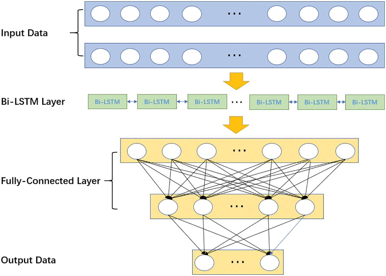
Figure 3: The structure of BL-FC model

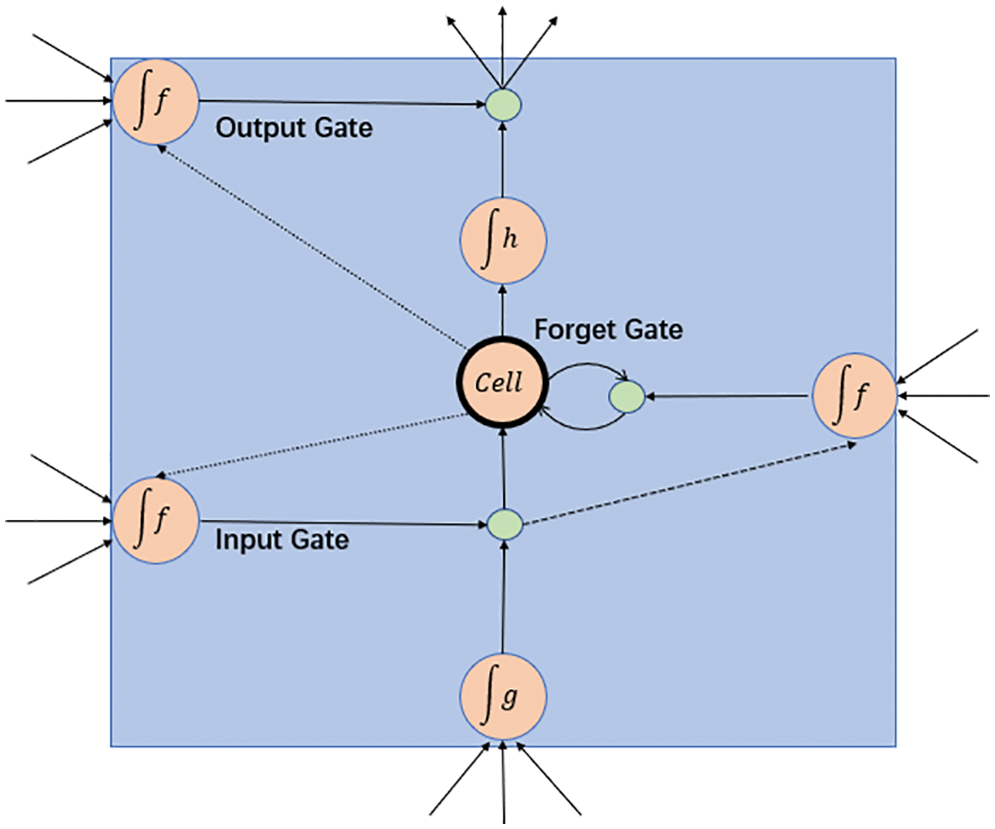
Figure 4: The structure of LSTM

it=σ(Wi⋅[ht−1,xt]+bi) (5)

ft=σ(Wf⋅[ht−1,xt]+bf) (6)

c~t=tanh⁡(Wc⋅[ht−1,xt]+bc) (7)

ct=ft∗ct−1+it∗c~t (8)

ot=σ(Wo⋅[ht−1,xt]+bo) (9)

ht=ot∗tanh(Ct) (10)

where it , ft , ot are input gate, forget gate, and output gate respectively and ht is the hidden state of t-th step. c~t represents the information stored in the previous LSTM cell, and ct is the memory cell currently. σ is the sigmoid function, which is used to map data between 0 and 1,

Eq. (5) is the formulation of input gate. By using a sigmoid function, this gate makes the decision of whether or not the new information will be added into the LSTM cell. Eq. (6) describes the working process of the forget gate. Forget gate can use sigmoid function to make the decision of what information should be removed from the LSTM cell, and the decision is mainly determined by the value of ht−1 and xt . Then by combing it , ft , c~t , we achieve the update of data in LSTM cell. The specific process is shown in Eq. (8). The last gate is output gate. Similar to the other two gates, it also uses a sigmoid function to decide what part of the information stored in the LSTM cell contributes to the output. Finally, a tanh function is used to map the values of output gate into –1 and 1.

From the formula above, we can conclude that by using these three gates, LSTM can preserve or discard pre-order data as needed. However, LSTM only preserves data in the forward direction, so the feature of sequence data can only be extracted and learned in one direction. This method ignores the important information from the backward direction. Therefore, when faced with abnormal temperatures, these LSTM-Based models often perform not that well. Bi-LSTM is the combination of two LSTM in opposite directions. It can preserve information of time series in two directions and enable additional training by traversing the input data twice. The final output of Bi-LSTM is also the combination of the forward and backward LSTM, which fully reflects the correlation between time series. Additional training and bidirectional feature extraction ensure that Bi-LSTM has better performance in the prediction of fluctuating temperature.

2.4 Procedure for BL-FC Model to Predict Temperature

The training and prediction procedure of BL-FC is described as follows:

Training input: Normalized and standardized data set X ;

Step 1: Use the sliding window method to construct the input data set into sample data set like matrix S , and target data set like matrix P .

Step 2: Determine parameters like units, learning rate, epoch, batch size, optimization algorithm, and the length of target and sample sequence, then build models on Keras.

Step 3: Train the model and validate it using the train set and validation set.

Step 4: Evaluate the prediction result of the model.

Training output: A trained temperature prediction model.

Prediction input: Test sample X ;

Prediction output: The predicted value Y corresponding to X .

3  Experiment

In this section, we will introduce our four experiments based on different time series prediction models and explain our performance metric and parameter settings.

3.1 Model Evaluation

Model evaluation refers to the process of using different performance metrics to evaluate the performance of models according to the specific situation. Appropriate performance metrics reveal the accuracy of the prediction result thoroughly, which is instructive to the construction and refinement of the model. Common performance metrics are RMSE, MSE, MAE. This paper utilizes MSE and MAE as performance metrics.

Note the mean value of the values to be fitted is yi and the value predicted is h(xi) .

Mean Squared Error (MSE) is the average of the squared error. The specific formula is shown in Eq. (11).

MSE=1M∑i=1M(h(xi)−yi)2 (11)

Mean Absolute Error (MAE) is the average of all absolute errors. The formula is shown in Eq. (12).

MAE=1M∑i=1M|h(xi)−yi| (12)

In simple terms, MSE is easy to calculate, and MAE is more robust to abnormal points.

3.2 Parameters

3.2.1 Time Series Length and Forecast Hours

According to the analysis in the experiment dataset, we can conclude that time series length and forecast hours are determined by the sample target ratio. In this paper, we adopt a 4:1 ratio uniformly. We designed four sets of experiments by changing the length of the time series in four different time series prediction models. The specific ratio of time series length and forecast hours are 16h:4h, 24h:6h, 32h:8h, and 40h:10h.

3.2.2 Learning Rate

Learning rate is a hyperparameter that controls how much to change the model in response to the estimated error each time the model weights are updated. An appropriate learning rate is crucial for finding the optimal weights of the model. A small learning rate may result in a long training process, whereas a large learning rate may lead to an unstable training process. In this paper, the initial learning rate is set to be 0.01 and automatically adjusted during the training process.

3.2.3 Parameters in BL-FC Model

There are also several parameters to be determined in the BL-FC model. The number of units in the Bi-LSTM module and fully connected module represents the dimensions of output data. Through experiments, the number of units in the first three layers are set to be 30, 20, 10 respectively.

The activation function is the basis for an artificial neural network to extract and learn complex features. These functions can bring non-linear properties to the network, which allow models to fit all kinds of data. Relu and Tanh are the two most commonly used activation functions. In general, Relu has a wider application range and a better performance. However, through experiments, our model performs best when using tanh on the Bi-LSTM layer and Relu on the fully connected layers.

Model optimization is the process of adjusting hyperparameters in order to minimize the cost function by using optimization algorithms. A good optimization algorithm can speed up the process of training and can even get a better result. In our experiment, the Adam algorithm with the fastest converge speed [25] is used.

Other parameters are determined through experiments. Epoch is set to be 30, the batch size is 100, and the ratio of the train set, validation set, and test set is 8:1:1.

3.3 Analysis of the Result

In order to show the superiority of our model, four experiments with different time series length and forecast hours are carried out on RNN, GRU, LSTM, and BL-FC model.

The prediction results of the four experiments are shown in Tab. 1.

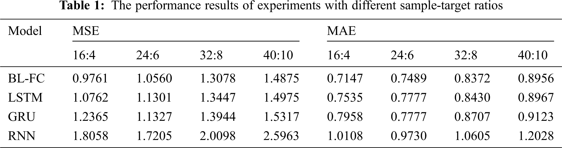
Just as we analyzed before, when facing long-term dependencies, RNN performs the worst among the four temperature prediction models. When the ratio of time series length and forecast hours is 40:10, the MSE and MAE of the temperature prediction result reach 2.5963 and 1.2028 respectively, which is far from the 1.4875 and 0.8956 predicted by BL-FC. It indicates that the model based on RNN is not suitable for temperature prediction.

Contrary to RNN-Based model, our BL-FC model outperforms other experimental models in every metric we adopt, followed by LSTM and GRU. When the time series length and forecast hours is set to 16:4, MSE and MAE reach 0.9761 and 0.7147 respectively, which is the best prediction result among all the experiments. As the ratio of time series length and forecast hours increases, although the advantage gradually decreases, BL-FC model still better than RNN, LSTM, and GRU-Based models.

In order to display the prediction results of the model intuitively, we randomly select the predicted value for 500 h and compare it with the actual temperature.

Figs. 5–8 are the line charts of the predicted and actual temperature for 500 consecutive hours, each of them uses a different time series length and forecast hours.

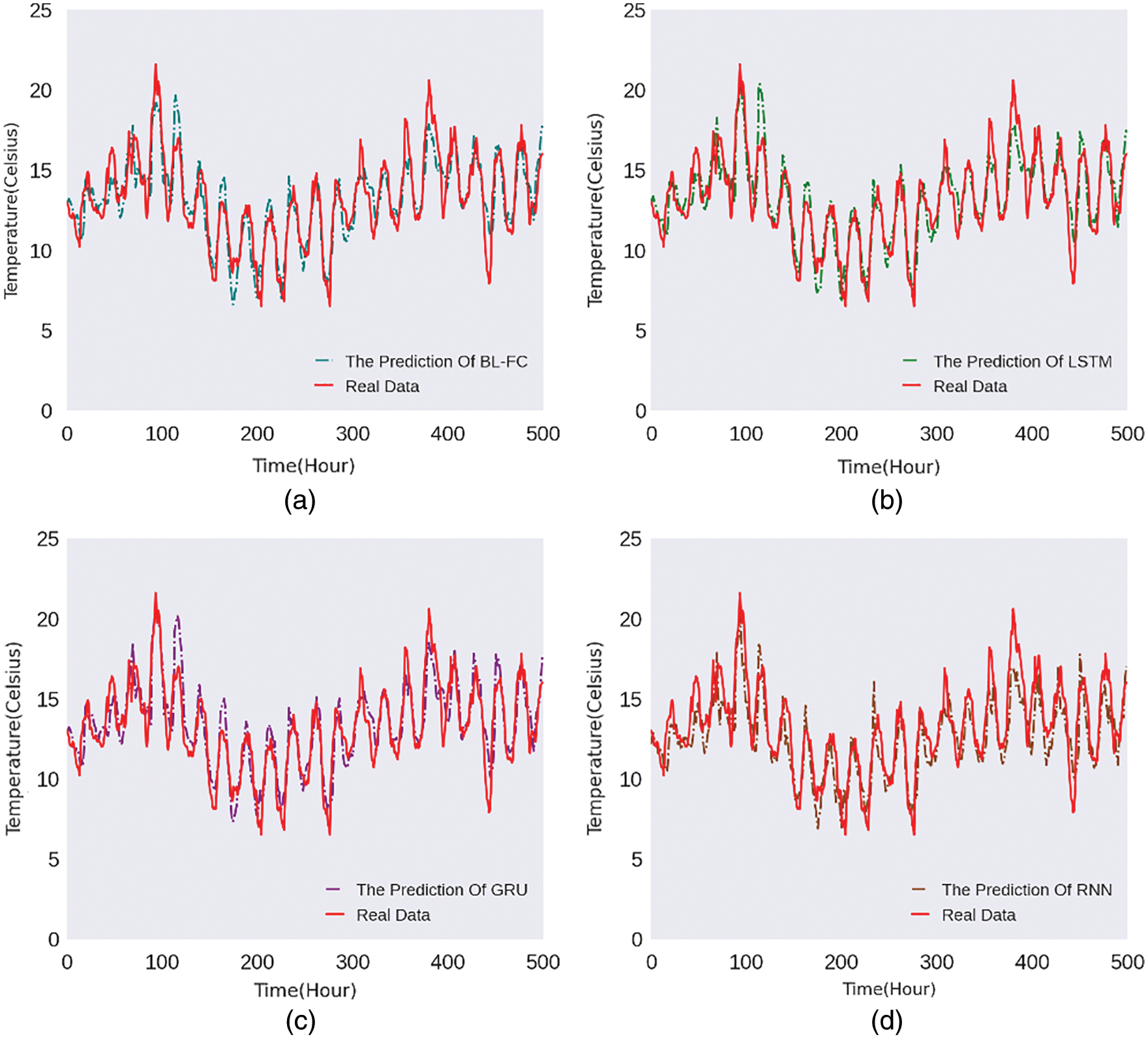
Figure 5: 16h:4h 500-hours temperature line chart

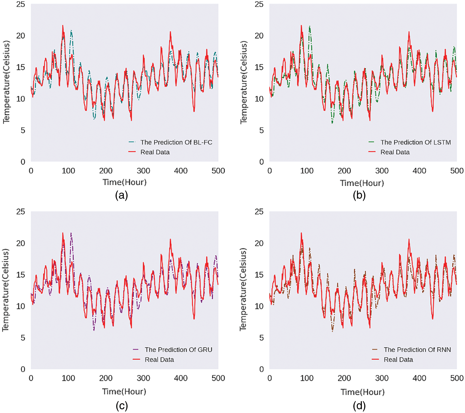
Figure 6: 24h:6h 500-hours temperature line chart

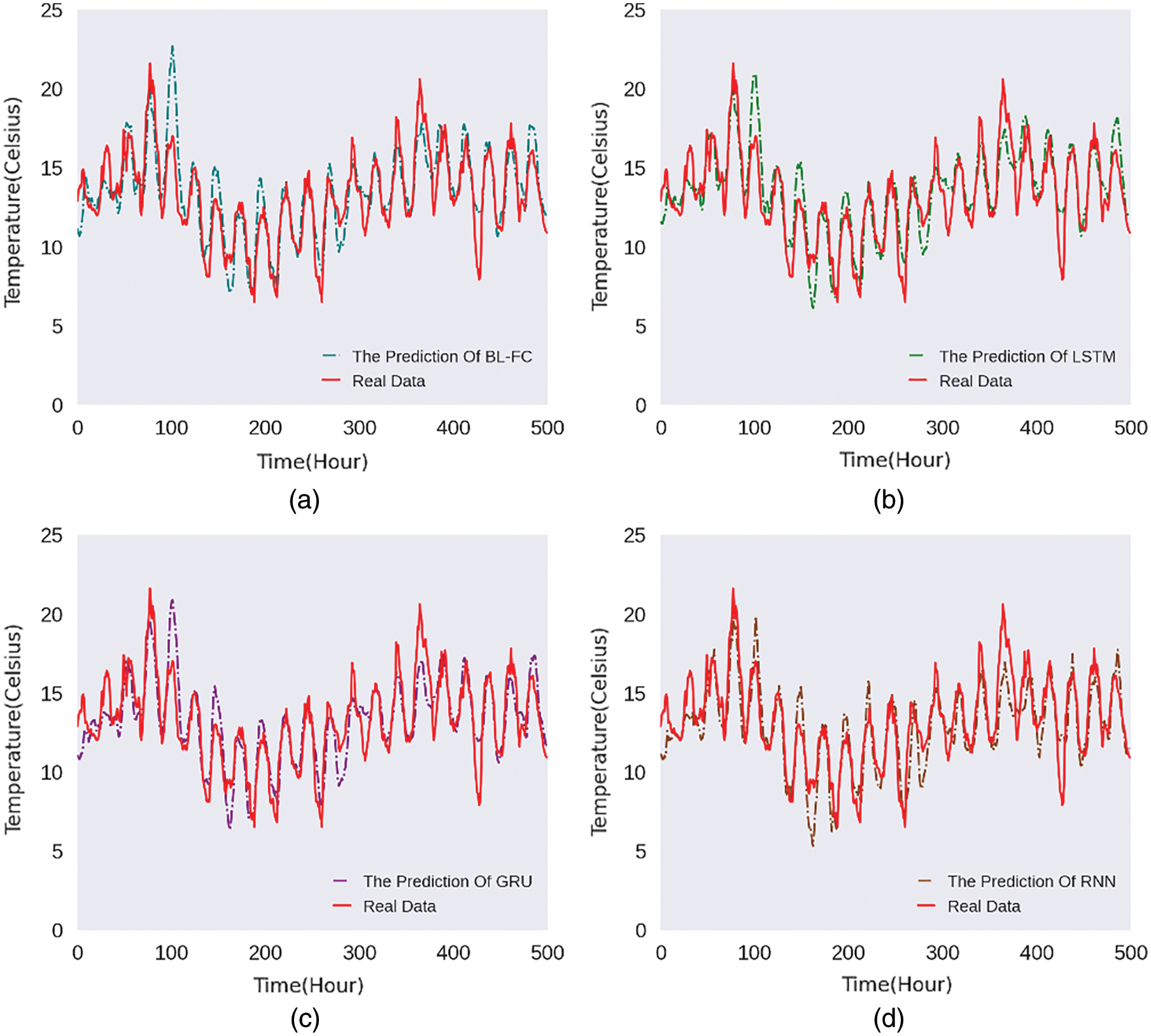
Figure 7: 32h:8h 500-hours temperature line chart

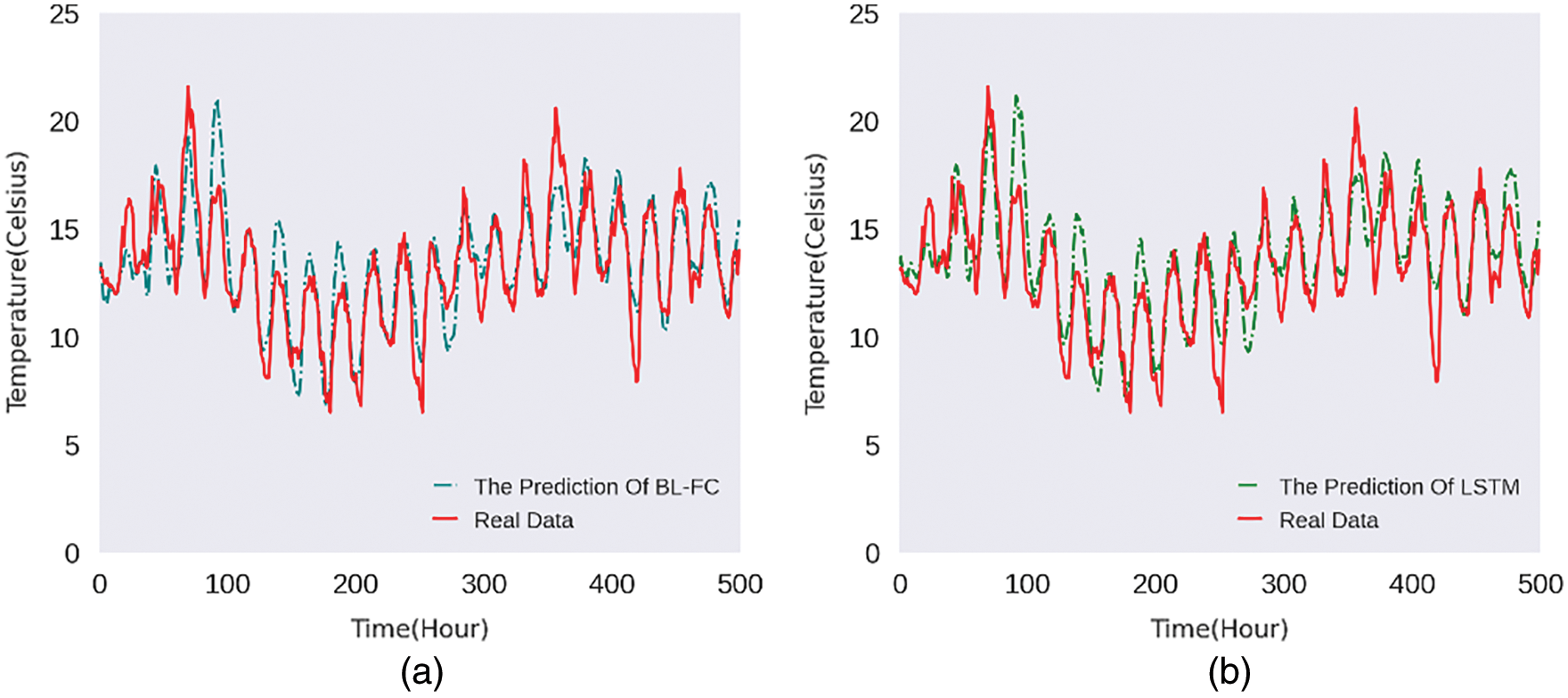
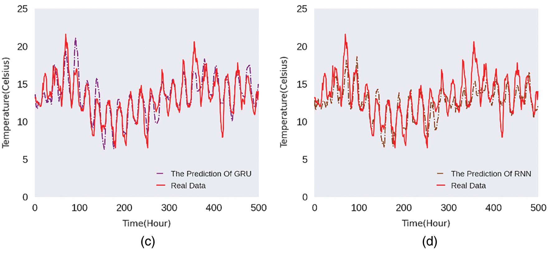
Figure 8: 40h:10h 500-hours temperature line chart

From Figs. 5–8, it can be seen that the four models all have a delay in the prediction of temperature changes, but BL-FC and LSTM-Based models respond to the changes quickly and have the smallest delay compared to the other two models. Besides, the prediction of abnormal temperature is also a major difficulty in temperature prediction. From the four figures above, we can conclude: BL-FC and LSTM-Based models have relatively small errors in the prediction of abnormal temperatures. Combining with the performance metrics shown in Tab. 1, we can see that our BL-FC is more suitable for temperature prediction than the other three models.

4  Conclusion

This paper proposes BL-FC short-term local temperature deep learning modeling method for complex meteorological system, which can make full use of massive meteorological data to build a more accurate model. In order to obtain the required sample data, the sliding window method is used to process 1981122 consecutive hour data of 15 meteorological factors provided by Mayo Weather Station. Then, the processed data is divided into training set, testing set, and validation set according to the ratio of 8:1:1. Based on these data, four typical deep learning models are studied, which are BL-FC, LSTM model, GRU model and RNN model. The experimental results show that the MSE and MAE of BL-FC are always superior to the other three models. Additionally, by comparing the prediction results of 500 consecutive hours of actual temperature data randomly selected, we can also see the advantages of BL-FC model: faster response to temperature changes and more accurate prediction of abnormal temperature. After determining the appropriate time series length and prediction hours, the BL-FC model can get accurate prediction results, and respond quickly when the temperature changes. Therefore, the temperature modeling method BL-FC can make use of meteorological big data to structure a more accurate local temperature prediction method, and make the model more accurate through continuous learning of data, which has a good application prospect in regional temperature prediction.

The length of prediction sequence selected in this study is 10. In further work, attention mechanism is introduced into our BL-FC model to further improve the accuracy of the model and predict regional long-term temperature. Moreover, the research method of this paper can be further applied to the prediction of other meteorological factors, so as to improve the accuracy of other factors and make the deep learning method better applied to the meteorological field.

Funding Statement: This work was supported by NUIST Students’ Platform for Innovation and Entrepreneurship Training Program (No. 202010300202) and the National Natural Science Foundation of China under Grant 62072251.

Conflicts of Interest: The authors declare that they have no conflicts of interest to report regarding the present study.

This work is licensed under a Creative Commons Attribution 4.0 International License, which permits unrestricted use, distribution, and reproduction in any medium, provided the original work is properly cited.