DOI:10.32604/iasc.2021.016491
| Intelligent Automation & Soft Computing DOI:10.32604/iasc.2021.016491 | |
| Article |
Control Charts for the Shape Parameter of Skewed Distribution
1Department of Statistics, Government Graduate College of Science, Wahdat Road, Lahore, Pakistan
2Department of Statistics, COMSATS University Islamabad, Lahore Campus, Lahore, Pakistan
3Institute of Business & Management, University of Engineering and Technology, Lahore, Pakistan
*Corresponding Author: Riffat Jabeen. Email: drriffatjabeen@cuilahore.edu.pk
Received: 03 January 2021; Accepted: 14 March 2021
Abstract: The weighted distributions are useful when the sampling is done using an unequal probability of the sampling units. The Weighted Power function distribution (WPFD) has applications in the fields of reliability engineering, management sciences and survival analysis. WPFD is more beneficial in Statistical process control (SPC). SPC is defined as the use of statistical techniques to control a process or production method. SPC tools and procedures can help to monitor process behaviour, discover problems in internal systems, and find solutions for production issues. To identify and remove the variation in different reliability processes and also to monitor the reliability of machines where the number of errors follows WPFD, we develop control charts to keep the process in control. A memory-based control chart like an exponentially weighted moving average (EWMA) control chart and an extended exponentially weighted moving average (EEWMA) control chart are discussed and compared each other. The proposal of these control charts is based on the modified maximum likelihood estimator (MMLE) under the shape parameter of WPFD. We have presented Monte Carlo simulation technique and a real-life application to compare the proposed control charts. This study shows that an EEWMA control chart based on MMLE performs better than EWMA control chart, when the underlying distribution of the errors in process monitoring follows WPFD. These findings can be useful for researchers and practitioners in dealing with production errors and optimizing the output.
Keywords: Weighted Power function distribution; EWMA control chart; EEWMA control chart; modified maximum likelihood estimator; management sciences; quality charts
The different production processes in industries face commonly two types of variations: common cause variation and special cause variation. Common cause variation always exists even if the process is designed very well and maintained very carefully. This variation should be relatively small in magnitude and is uncontrollable and due to many small unavoidable causes. A process is said to be in statistical control if only common cause variation is present. The variations outside this common cause pattern are called special cause variations. These variations are subject to some problem in the system, like the poor tuning of equipment, controller fell asleep or got absent, the computer stopped working, a poor lot of raw material, machine break down. A process working under both types of variation is said to be out of control.
These variations may affect the production process and ultimately result in a defective output. The consequences of it are pretty severe. Companies have to face high cost as well as their reputation will be at stake. Therefore, in order to avoid variations in the process, there is a need to use control charts to keep the process under control. Zaka et al. [1] introduced a new class of distribution called WPFD in order to have more application in applied sciences such as biosciences engineering, management sciences. The weighted distributions are helpful when the sampling is done using an unequal probability of the sampling units. WPFD is more useful in Statistical process control. Statistical process control (SPC) is defined as the use of statistical techniques to control a process or production method. SPC tools and procedures can help to monitor process behavior, discover issues in internal systems, and find solutions for production problems. Two types of control charts are commonly studied, memory less control chart i.e., Shewhart control chart and memory based control charts such as EWMA and HEWMA etc. Many works have been done in this regard, such as the EWMA control charts firstly by Roberts [2], and recently by Li et al. [3] and Nguyen et al. [4]. The cumulative-sum (CUSUM) control charts firstly by Page [5], Sanusi et al. [6], Haq et al. [7] and Hossain et al. [8]. The mixed EWMA-CUSUM control charts by Abbas et al. [9], Ajadi and Riaz [10]. The hybrid exponential weighted moving average (HEWMA) control charts due to Shamma et al. [11] and Haq [12].
In real life scenario, this is not always possible to fulfil the normality assumption for the distribution of error during the process. A very few works in literature is about this situation of not normal process distribution including Noorossana et al. [13], Lin et al. [14], Erto et al. [15], Liang et al. [16] and Ahmed et al. [17]. The EWMA statistic is widely used for shift detection in the ongoing process either to monitor qualitative or quantitative physical phenomena. The generalized form of the existing EWMA statistic was introduced by Naveed et al. [18] and named it as EEWMA.
2 The Conventional EWMA Control Chart
Let the distribution of the underlying process having the sequence {Xt} is normal. Also, let the
The smoothing constant
3 The Traditional Extended Exponentially Weighted Moving Averages Control chart
When the distribution of the process is normal, the EEWMA control chart was introduced by Naveed et al. [18]. The EEWMA control chart by Naveed et al. [18] is given as
where
The mean and variance are given as
And
4 Proposed Extended Exponentially Weighted Moving Averages Control Chart Under Non-Normality
Following Zaka et al. [1], it is assumed that the process random variable
and
Modified Maximum Likelihood Estimator (MMLE) is used to construct memory less and memory-based control charts to monitor the shape parameter of a process that follows a WPFD. The estimator for the shape parameter of WPFD defined by Zaka et al. [1] is given as,
The variance of the
Now using Zaka et al. [1] and Naveed et al. [18], the EEWMA statistic is given as
For t = 1
For t = 2
Let
Let
By taking expectation, we get
Replacing
By using geometric series, we get
So,
Let
Let
The control limits are given as
a) Generate a random sample of size n = 150 on “Xt” from the WPFD are
b) Compute
c) Repeat steps (a) and (b), for 5000 times and compute
d) Repeat step (c) for 5000 times and compute
e) Compute control limits to construct EEWMA control charts based on
f) Compute ARL value for each EEWMA control chart that based on
g) Now fix ARL0 = 500 for in-control state of the process and search the suitable value of L, so that ARL0 for in-control state of process is achieved.
h) Now assume if the process parameter “
i) Plot ARLs values against the values of shift that used in step (g) and (h).
j) It is to note that the procedure of EWMA control chart based on
k) Repeat this process 5000 times to obtain the ARLs, SDRLs and percentiles.
We consider the average run length to compare the performance of the proposed estimators. It is taken as the average number of samples that are used before as the process is out of control. ARL0 indicates the in control ARL, while the ARL1 describes the out of control ARL. A chart having a larger ARL0 and smaller ARL1 is considered better to be used for the process monitoring.
The Tabs. 1–3 is constructed for ARL values when the parameters of underlying process following WPFD using EWMA and EEWMA. Figs. 1–3 presents the ARL values for EWMA and EEWMA. We observed that EEWMA control chart detects earlier on small shifts as compare to EWMA control chart for different choices of
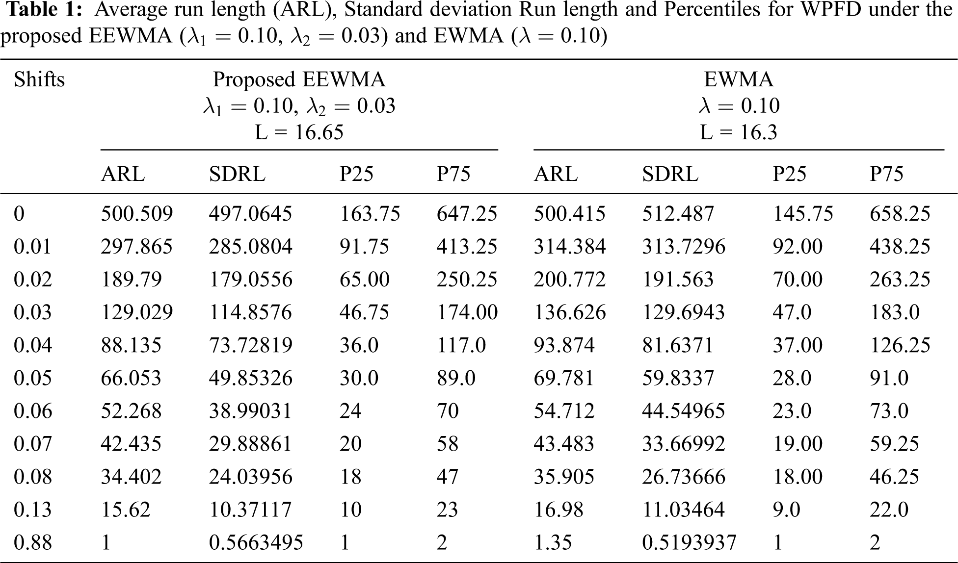

Figure 1: ARL for the shape parameter of WPFD using EWMA and EEWMA
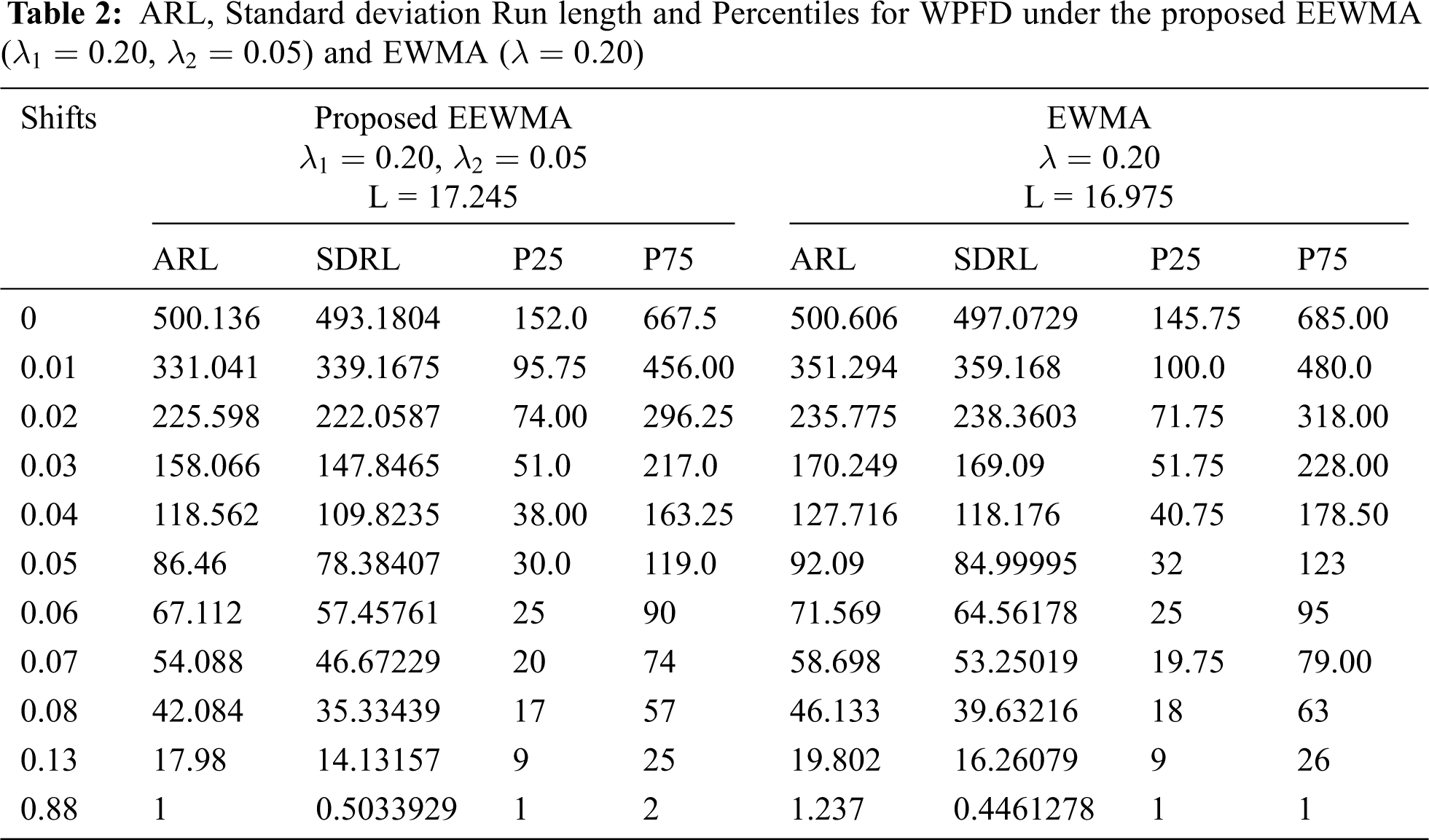

Figure 2: ARL for the shape parameter of WPFD using EWMA and EEWMA
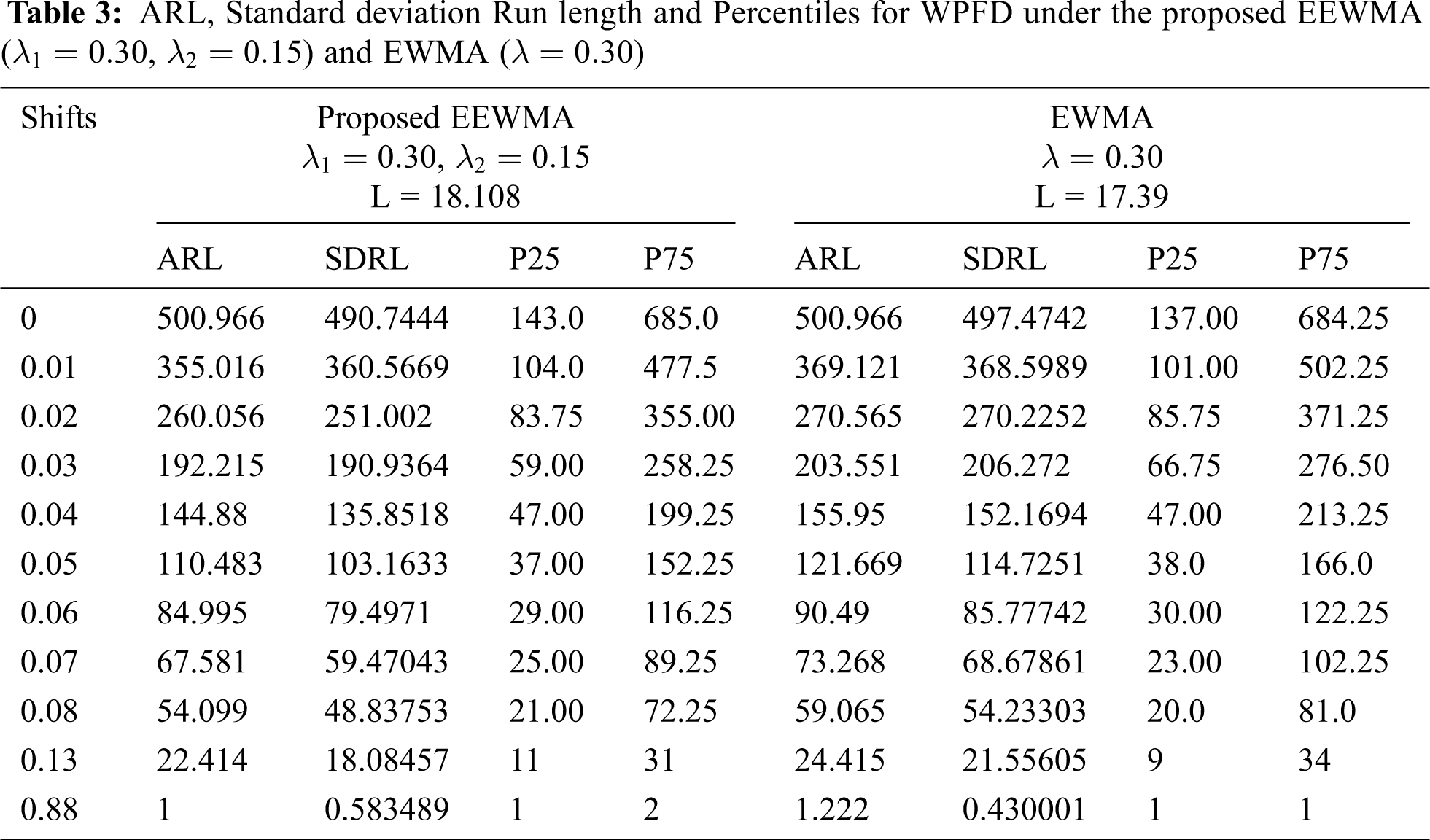

Figure 3: ARL for the shape parameter of WPFD using EWMA and EEWMA
In order to see the working procedure of the proposed control charts, a simulation study was carried out. For this purpose, we generated 25 observations from a WPFD for in-control process, and the next 25 observations were generated from the shifted process with 0.01. The estimated values of the proposed EWMA statistic under MMLE were computed for the selected levels of the proposed control charts parameters with
In Fig. 5, we noted that the proposed EEWMA control chart under MMLE detected a shift at the 32th sample, while in Fig. 4; the EWMA control chart under MMLE could not detect the shift. Hence, this shows that the proposed EEWMA control chart under MMLE has a greater ability to detect smaller shifts earlier, as compared to the EWMA control chart.
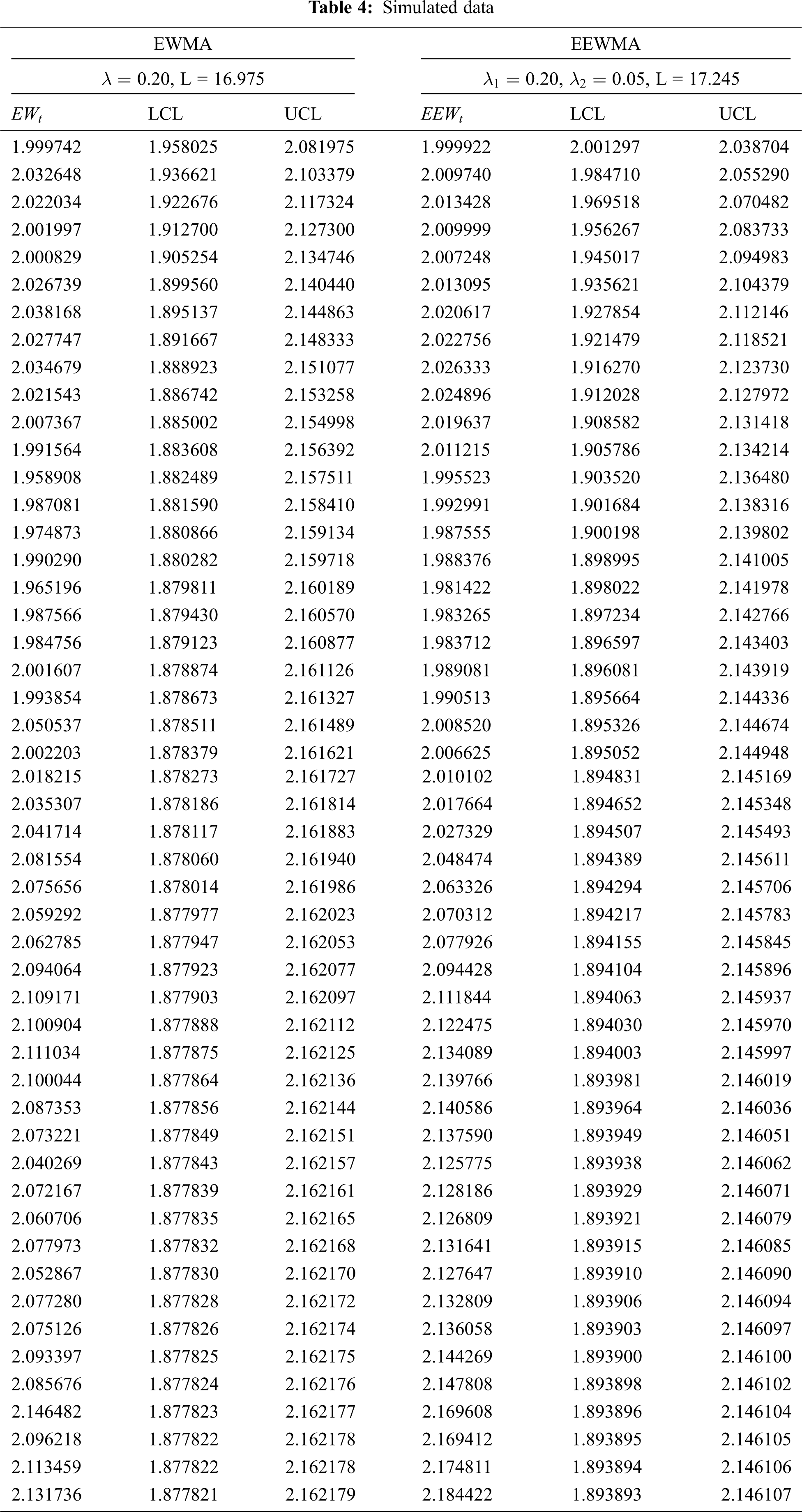
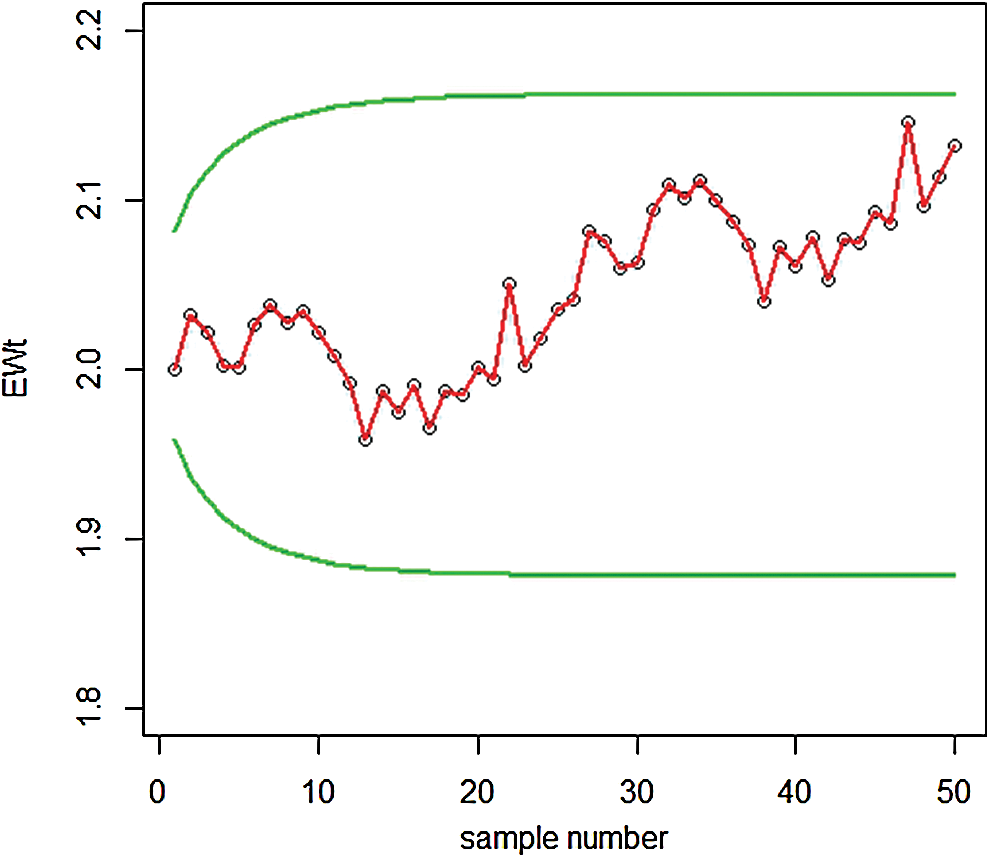
Figure 4: Graph of simulated data of the proposed EWMA control chart under MMLE
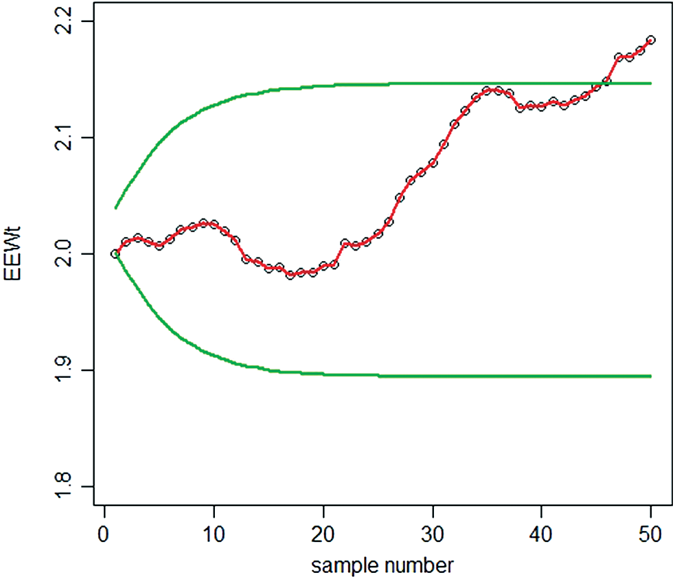
Figure 5: Graph of simulated data of the proposed EEWMA control chart under MMLE
We have discussed the process monitoring for WPFD. In real life, we may face the situation that any specific process does not follow the normal distribution. But the distribution of the errors in the process becomes WPFD. In the current work, we first estimate the parameters of the distribution of the errors during any process by using MMLE, which was claimed better to estimate the parameters of WPFD. By using the MMLE, we then modified the quality control charts used in literature, such as EWMA and EEWMA control charts. We see that EEWMA control chart under MMLE can be used to monitor the process when the underlying distribution of the errors in process monitoring follows WPFD. It is therefore hoped that the findings of this study will be useful for researchers in different fields of applied sciences. It will be helpful to identify the error in time and making strategies to deal with it. Companies can control their cost and improve product quality by applying the proposed quality chart processes.
Funding Statement: The authors received no specific funding for this study.
Conflicts of Interest: The authors declare that they have no conflicts of interest to report regarding the present study.
1. A. Zaka, A. S. Akhter and R. Jabeen, “Asymmetry approach to study for chemotherapy treatment and devices failure time’s data using modified Power function distribution with some modified estimators,” International Journal of Computing Science and Mathematics, (Accepted Paper),2020.https://www.inderscience.com/info/ingeneral/forthcoming.php?jcode=ijcsm. [Google Scholar]
2. S. W. Roberts, “Control chart tests based on geometric moving averages,” Technometrics, vol. 1, pp. 239–250, 1959. [Google Scholar]
3. Z. Li, M. Xie and M. Zhou, “Rank-based EWMA procedure for sequentially detecting changes of process location and variability,” Quality Technology and Quantitative Management, vol. 15, no. 3, pp. 354–373, 2018. [Google Scholar]
4. H. D. Nguyen, K. P. Tran and C. Heuchenne, “Monitoring the ratio of two normal variables using variable sampling interval exponentially weighted moving average control charts,” Quality and Reliability Engineering, vol. 35, no. 1, pp. 439–460, 2019. [Google Scholar]
5. E. S. Page, “Continuous inspection scheme,” Biometrika, vol. 41, no. 1, pp. 100–115, 1954. [Google Scholar]
6. R. A. Sanusi, M. Riaz and N. Abbas, “Combined Shewhart CUSUM charts using auxiliary variable,” Computers and Industrial Engineering, vol. 105, pp. 329–337, 2017. [Google Scholar]
7. A. Haq and W. Munir, “Improved CUSUM charts for monitoring process mean,” Journal of Statistical Computation and Simulation, vol. 88, no. 9, pp. 1684–1701, 2018. [Google Scholar]
8. M. P. Hossain, R. A. Sanusi, M. H. Omar and M. Riaz, “On designing Maxwell CUSUM control chart: An efficient way to monitor failure rates in boring processes,” International Journal of Advanced Manufacturing Technology, vol. 100, no. 5–8, pp. 1923–1930, 2019. [Google Scholar]
9. N. Abbas, M. Riaz and R. J. M. M. Does, “Mixed exponentially weighted moving average-cumulative sum charts for process monitoring,” Quality and Reliability Engineering International, vol. 29, no. 3, pp. 345–356, 2013. [Google Scholar]
10. J. O. Ajadi and M. Riaz, “Mixed multivariate EWMA-CUSUM control charts for an improved process monitoring,” Communications in Statistics Theory and Methods, vol. 46, no. 14, pp. 6980–6993, 2017. [Google Scholar]
11. S. E. Shamma and A. K. Shamma, “Development and evaluation of control charts using double exponentially weighted moving averages,” International Journal of Quality and Reliability Management, vol. 9, no. 6, pp. 18–25, 1992. [Google Scholar]
12. A. Haq, “A new hybrid exponentially weighted moving average control chart for monitoring process mean,” Quality and Reliability Engineering International, vol. 29, pp. 1015–1025, 2013. [Google Scholar]
13. R. Noorossana, S. Fathizadan and M. R. Nayebpour, “EWMA Control Chart performance with estimated parameters under non-normality,” Quality Technology and Quantitative Management, vol. 32, no. 5, pp. 1638–1654, 2016. [Google Scholar]
14. Y. C. Lin, C. Y. Chou and C. H. Chen, “Robustness of the EWMA median control chart to non- normality,” International Journal of Industrial and Systems Engineering, vol. 25, no. 1, pp. 35–58, 2017. [Google Scholar]
15. P. Erto, G. Pallotta, B. Palumbo and C. M. Mastrangelo, “The performance of semi empirical bayesian control charts for monitoring Weibull data,” Quality Technology and Quantitative Management, vol. 15, no. 1, pp. 69–86, 2018. [Google Scholar]
16. W. Liang, D. Xiang, X. Pu, Y. Li and L. Jin, “A robust multivariate sign control chart for detecting shifts in covariance matrix under the elliptical directions distributions,” Quality Technology and Quantitative Management, vol. 16, no. 1, pp. 113–127, 2019. [Google Scholar]
17. A. Ahmed, A. Sanaullah and M. Hanif, “A robust alternate to the HEWMA control chart under non-normality,” Quality Technology and Quantitative Management, vol. 17, no. 4, pp. 423–447, 2019. [Google Scholar]
18. M. Naveed, M. Azam, N. Khan and M. Aslam, “Design of a control chart using extended EWMA statistic,” Technologies, vol. 6, no. 108, pp. 2–15, 2018. [Google Scholar]
 | This work is licensed under a Creative Commons Attribution 4.0 International License, which permits unrestricted use, distribution, and reproduction in any medium, provided the original work is properly cited. |