DOI:10.32604/iasc.2021.017920
| Intelligent Automation & Soft Computing DOI:10.32604/iasc.2021.017920 | |
| Article |
Energy-Efficiency Model for Residential Buildings Using Supervised Machine Learning Algorithm
1School of Computer Science, National College of Business Administration and Economics, Lahore, 54000, Pakistan
2Center for Cyber Security, Faculty of Information Science and Technology, Universiti Kebansaan Malaysia (UKM), 43600, Bangi, Selangor, Malaysia
3School of Information Technology, Skyline University College, University City Sharjah, 1797, Sharjah, UAE
4Department of Computer Science, Lahore Garrison University, Lahore, 54000, Pakistan
5Canadian University Dubai, Dubai, UAE
6Riphah School of Computing & Innovation, Faculty of Computing, Riphah International University, Lahore, 54000, Pakistan
7Pattern Recognition and Machine Learning Lab, Department of Software Engineering, Gachon University, Seongnam, 13557, Korea
8School of Computer Science, Minhaj University Lahore, Lahore, 54000, Pakistan
*Corresponding Author: Muhammad Adnan Khan, Email: adnan.khan@riphah.edu.pk
Received: 17 February 2021; Accepted: 15 May 2021
Abstract: The real-time management and control of heating-system networks in residential buildings has tremendous energy-saving potential, and accurate load prediction is the basis for system monitoring. In this regard, selecting the appropriate input parameters is the key to accurate heating-load forecasting. In existing models for forecasting heating loads and selecting input parameters, with an increase in the length of the prediction cycle, the heating-load rate gradually decreases, and the influence of the outside temperature gradually increases. In view of different types of solutions for improving buildings’ energy efficiency, this study proposed a Energy-efficiency model for residential buildings based on gradient descent optimization (E2B-GDO). This model can predict a building’s heating-load conservation based on a building energy performance dataset. The input layer includes area (distribution of the glazing area, wall area, and surface area), relative density, and overall elevation. The proposed E2B-GDO model achieved an accuracy of 99.98% for training and 98.00% for validation.
Keywords: Heating-load prediction; machine learning; gradient descent optimization
Buildings need to be designed to support people’s health and well-being and to use the least amount of materials and resources. This applies to the construction of new buildings as well as the improvement of existing ones. In performance-driven building design, simulation is used to understand a building’s energy consumption [1]. This approach is known as Building performance simulation (BPS), and it allows a designer to examine in advance the influence of a building’s shape, materials, and systems on its expected thermal output. The search for an optimal design via simulation has conventionally had a small search space and a narrow region of possible choices. However, optimization, which can improve efficiency, can help to dramatically expand the search space during the design of a product [2].
The advantages of search optimization are realized when the optimization routine can assess thousands of possible options. However, large runs of realistic performance simulations require significant time and resources. Optimization can reduce the amount of specialist labor needed to scan broad additional spaces, but the resulting computational load can be daunting. Surrogate or data-driven models are based on mathematical inputs learned from measured or virtual data related to physical properties. For instance, the thermophysical properties of building materials and environmental-condition parameters can be used to predict indoor environmental conditions. Sufficiently accurate surrogate models, therefore, can provide fast, precise alternatives to performance simulators. It has been suggested that such models are superior to random forest, support vector machines, and decision trees for forecasting the hourly energy demand of buildings [3].
Buildings account for one-third of the world’s overall electricity consumption. Although energy efficiency standards are important instruments for improving buildings’ energy efficiency, the criteria can vary from country to country. The energy standard used in the US has saved more than $56 billion in electricity costs. Meanwhile, china requires new buildings to be 65% more energy efficient than they were in the 1980s. Energy efficiency standards in the EU tend to focus more on existing buildings. In India, the energy conservation building code for large-scale commercial buildings was adopted in 2007 [1,4].
Improvements to global energy efficiency have been slowing down since 2015. Energy Efficiency 2019, which tracks trends in global energy efficiency, has investigated the factors related to this recent slowdown while also emphasizing how digitization can improve energy efficiency [2]. In digitization, the input layer consists of a sphere, which can be described as a flat circle or the space that occupies an object’s surface. This area is measured in units per square centimeter, in square feet, and in square inches [3].
When installing glass in a structure, the area of the wall framing the glass is measured using the standard equation, which is height × length [4]. The surface-to-volume (S/V) ratio (the circumference’s three-dimensional magnitude-area ratio) is a crucial factor for determining heat loss/gain. The larger the surface area, the higher the heat. Low S/V ratios, therefore, reflect minimal heat gain and minimal heat loss [5]. Reducing compactness ratios for heating and cooling buildings can reduce costs and improve efficiency [6]. Most heating and cooling loads are worsened when the building’s thermal load is 25°C, its cooling load temperature is 30°C, and the outputs are below 16°C [7].
Energy included in the UN Environment Program includes climate construction, building envelopes, building services, and energy systems. The temperature created inside a building is estimated at 19°C, according to the researchers [8]. Buildings have large surface areas and high volume. The main thermal envelope area and its volume (ratio A/V) represent the ratio between a building’s compactness and its expression; the thermal envelope separates the indoor and outdoor surroundings.
There are various thermal envelope characteristics under different climatic conditions, which have different effects on building management processes [9,10]. The US Environmental Protection Agency has described “low energy consumption as energy quality.” A study in France noted a clear association between energy consumption and size coefficients; if the relationship between building size and energy consumption is adjusted to climate change, its output generates very hot or very cold charges [11]. Development of energy consumptions varies according to temperature rather than the main effects of the glazed region, depending on the orientation of the building and annual energy demands. Various studies have investigated designing for different environments [12,13]. There are three types of relative compactness: window ratios, wall ratios, and glazing, as defined by the solar heat gain coefficient. Other factors, meanwhile, greatly affect the color of the facade of a building. Some structures can be made related to energy generation, the prevention of excessive heat, heat transfer, solar radiation absorption, and compactness [14–16].
Many studies have relied on mathematical models to calculate buildings’ heating efficiency. This approach is suitable for residential buildings but not commercial buildings because of inherent limitations [12,17]. Simulation techniques are mainly used for office buildings where the size of the rectangle L gives the building size at the total annual capacity. Just two building shapes have been studied in previous studies, but instead of heating the space to display the size of the house, its percentage is discussed, along with the relative compactness and glazing styles. The system model needs a low refrigeration load and low total building energy consumption [13,18].
This study investigated the key relationship for most apartments between convex ratio and building power efficiency and discusses the three major levels of convexity. The shape of the building has a direct effect on the building’s energy consumption. This study analyzes the impact of the curved shapes on the final energy demand by studying three different shapes. The differences in shape between the buildings was found to have an impact and on the final energy demand. Both amounts are less convex in the volumes of the curve, higher energy efficiency, and convexity of the direct mean [19,20]. Computational intelligence approaches, such as a fuzzy logic, artificial neural networks, and support vector machines, are robust approaches for future forecasting and prediction purposes [21–23].
3 Proposed E2B-GDO System Model
This study proposes a building energy-efficiency model based on gradient descent optimization (E2B-GDO) to forecast the energy performance of residential buildings. In this model, five layers are pushed toward the cloud if accuracy is achieved to conduct further processing for the validation phase (Fig. 1). The proposed model has 786 samples. Relative compactness, field, and overall height are inputs; heating and cooling loads are outputs. A cloud was used to store data, whether for testing or training. The model collects data from the cloud for the validation process. Trained data or inputs are fed into the cloud, which determines the evaluation system for testing purposes. Data are fed into the cloud and forwarded to the preprocessor layer, which will boost errors and missing values. Forwarding to the final iteration is the last step. The sensory layer is taken as an input layer providing inputs during the training process. The object layer selects the desired data from multiple data and selects the accurate data needed for the missing values in the preprocessing layer and normalizes the result to get an accurate raw data result. The prediction layer used Gradient descent optimization (GDO) to predict the outcome. Consistency is tested in the consistency layer regarding whether its accuracy is adequate, and the miss rate is verified. If the accuracy meets the requirement, it is moved to the cloud, and the process is repeated until all errors have been removed. Once errors are removed, the process moves to the validation phase, where it moves from the sensory layer to preprocessing. If the result is accurate, the final model is obtained; if not, it moves back to the sensory layer and repeats the process.
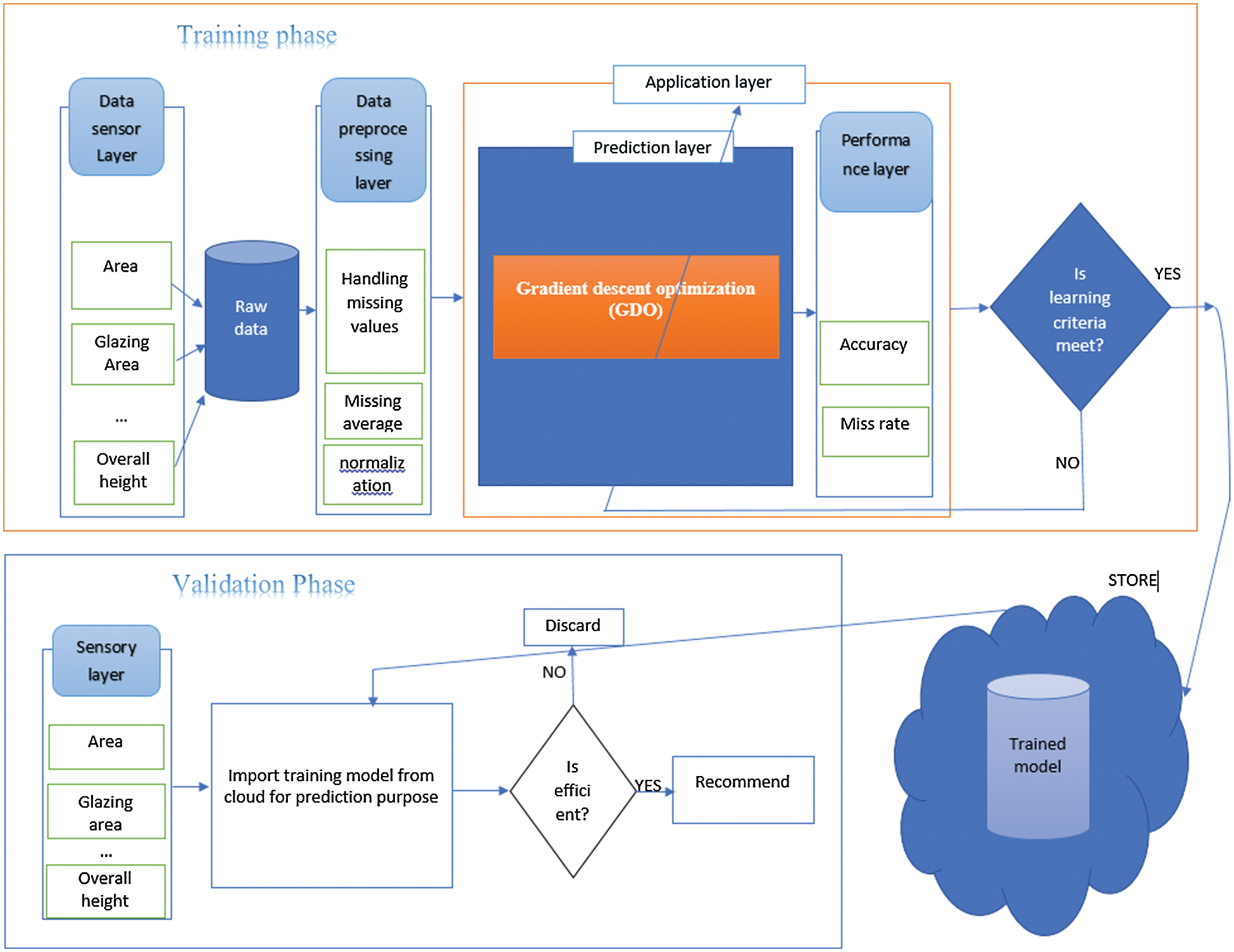
Figure 1: Proposed E2B-GDO system model
In the proposed model’s input layer, the hidden layer and output layer are used for computation and optimization through the backpropagation algorithm. Different steps are involved in the backpropagation algorithm, such as weight initialization, feedforward, error backpropagation, and weight and bias updating. Each neuron is given the activation function in a hidden layer, such as S(y) = alpha(y). The alpha function was used in the input layer shown in Eq. (2). The sigmoid activation function used in the output layer is given in Eq. (2).
We know the equation of the line is
where j = 1, 2, 3……n.
The second input taken for the output layer is shown in Eq. (3):
The output is shown in Eq. (4):
where k = 1, 2, 3…r.
The error involved in backpropagation is shown in Eq. (5):
where
The change of weights in the output is shown in Eq. (6):
Apply the chain rule method in Eq. (6):
After obtaining the value from Eq. (7), the weights are as shown in Eq. (8):
where
Updating the weight and bias between the output and hidden layer is as shown in Eq. (10):
At the input layer and hidden layer, updating the weights and bias are as shown in Eq. (11):
3.2 Proposed E2B-GDO System Model Using Fitness Modeling
Two layers of a feed-forward network are used in the GDO fitting application. A fitting network is used to train the selected data. Then, those data are divided into training, validation, and testing sets to define the architecture of the network. The Levenberg–Marquardt algorithm was used to train and fit 786 sets of data, randomly divided into 70% for training (538 samples), 15% for validation (115 samples), and 15% for testing (115 samples).
3.3 Proposed E2B-GDO Using Time-Series Modeling
The time-series standard was used to solve the three types of nonlinear problems using the dynamic network in GDO. The GDO time series was trained by first selecting and then dividing the data into training, validation, and testing sets to define the architecture of the network. MATLAB was used to train and fit 786 sets of data using a Nonlinear autoregressive exogenous model (NARX). Three layers were used in the time-series model, with a sensory layer as the input, a hidden layer as the prediction layer, and a performance layer that shows the output if the result is accurate. In the case of errors, the process is repeated.
MATLAB was used for the clone of the result. Tab. 1 shows the accuracy, missing rate in the training and the validation phase.

In Tab. 1, along with the comparison of previous approaches, performance is checked using a fitting model and a time series [14]. Tab. 1 shows a comparison of the accuracy and missing rate in training and validation for two kinds of approaches.
Tab. 2 shows the evaluation and prediction of residential buildings’ energy performance using the proposed E2B-GDO model and compares the results with those of other approaches, such as random forest and decision trees. The comparison is based on the factors of heating-load prediction based on building energy performance; the table also shows statistical measures such as accuracy, missing rate, and mean square error. The proposed E2B-GDO model was found to perform better than the other methods with regard to accuracy and MSE.

This study investigated buildings’ energy consumption and heat production using gradient descent optimization to predict heating and cooling load. The proposed Energy-efficiency model for residential buildings based on gradient descent optimization (E2B-GDO) can predict a building’s heating-load conservation based on a building energy performance dataset. The proposed E2B-GDO model achieved accuracies of 99.98% in training and 98.00 in validation. Area, relative compactness, and overall height have a significant effect on heating and cooling load. This study’s method can be applied to designing buildings to optimize energy performance for any given input variable based on either experimental or simulated data.
Acknowledgement: We thank our families and colleagues for their moral support.
Funding Statement: The author(s) received no specific funding for this study.
Conflicts of Interest: The authors declare that they have no conflicts of interest to report regarding the present study.
1. L. Pérez-Lombard, J. Ortiz and C. Pout, “A review on buildings energy consumption information,” Energy and Buildings, vol. 40, no. 3, pp. 394–398, 2008. [Google Scholar]
2. C. Huang, A. Zappone, G. C. Alexandropoulos, M. Debbah and C. Yuen, “Reconfigurable intelligent surfaces for energy efficiency in wireless communication,” IEEE Transactions on Wireless Communications, vol. 18, no. 8, pp. 4157–4170, 2019. [Google Scholar]
3. N. Dudley, Guidelines for applying protected area management categories. Iucn, 2008. [Google Scholar]
4. A. Ghaffarian, U. Berardi, A. Hoseini and N. Makaremi, “Intelligent facades in low-energy buildings,” British Journal of Environment and Climate Change, vol. 2, no. 4, pp. 437–448, 2012. [Google Scholar]
5. I. Danielski, M. Fröling and A. Joelsson, “The impact of the shape factor on final energy demand in residential buildings in nordic climates,” World Renewable Energy Conference, vol. 3, no. 1, pp. 4260–4264, 2012. [Google Scholar]
6. A. A. Anzi, D. Seo and M. Krarti, “Impact of building shape on thermal performance of office buildings in Kuwait,” Energy Conversion and Management, vol. 50, no. 3, pp. 822–828, 2009. [Google Scholar]
7. S. Abbas, M. A. Khan, L. E. F. Morales, A. Rehman, Y. Saeed et al., “Modeling, simulation and optimization of power plant energy sustainability for iot enabled smart cities empowered with deep extreme learning machine,” IEEE Access, vol. 8, no. 1, pp. 39982–39997, 2020. [Google Scholar]
8. A. J. Khalil, A. M. Barhoomm, B. S. A. Nasser, M. M. Musleh and S. S. A. Naser, “Energy efficiency predicting using artificial neural network,” International Journal of Academic Pedagogical Research (IJAPR), vol. 9, no. 3, pp. 1–7, 2019. [Google Scholar]
9. A. Tsanas and A. Xifara, “Accurate quantitative estimation of energy performance of residential buildings using statistical machine learning tools,” Energy and Buildings, vol. 49, pp. 560–567, 2012. [Google Scholar]
10. Z. Yu, F. Haghighat, B. C. Fung and H. Yoshino, “A decision tree method for building energy demand modeling,” Energy and Buildings, vol. 42, no. 10, pp. 1637–1646, 2010. [Google Scholar]
11. T. Nigitzand and M. Golles, “A generally applicable, simple and adaptive forecasting method for the short-term heat load of consumers,” Applied Energy, vol. 241, pp. 73–81, 2019. [Google Scholar]
12. X. J. Luo, L. O. Oyedele, A. O. Ajayi, C. G. Monyei, O. O. Akinade et al., “Development of an iot-based big data platform for day-ahead prediction of building heating and cooling demands,” Advanced Engineering Informatics, vol. 4, no. 2, pp. 23–36, 2019. [Google Scholar]
13. S. Seyedzadeh, F. Pour Rahimian and P. Rastogi, “Tuning machine learning models for prediction of building energy loads,” Sustainable Cities and Society, vol. 20, no. 4, pp. 1–14, 2019. [Google Scholar]
14. L. Yakai, T. Zhe and P. Peng, “Gmm clustering for heating load patterns in-depth identification and prediction model accuracy improvement of district heating system,” Energy and Buildings, vol. 190, no. 4, pp. 49–60, 2019. [Google Scholar]
15. R. Niemierko, Töppel, Jannick and Tränkler and Timm, “A divine copula quantile regression approach for the prediction of residential heating energy consumption based on historical data,” Applied Energy, vol. 10, no. 14, pp. 233–234, 2019. [Google Scholar]
16. D. S. Kapetanakis, E. Mangina and D. P. Finn, “Input variable selection for thermal load predictive models of commercial buildings,” Energy and Buildings, vol. 137, no. 17, pp. 13–26, 2017. [Google Scholar]
17. S. S. Roy, R. Roy and V. E. Balas, “Estimating heating load in buildings using multivariate adaptive regression splines, extreme learning machine, a hybrid model of MARS and ELM,” Renewable & Sustainable Energy Reviews, vol. 17, no. 3, pp. 52–68, 2017. [Google Scholar]
18. P. Potočnik, E. Strmčnik and E. Govekar, “Linear and neural network-based models for short-term heat load forecasting,” Strojniski Vestnik, vol. 9, no. 61, pp. 543–550, 2015. [Google Scholar]
19. K. M. Powell, A. Sriprasad, W. J. Cole and T. F. Edgar, “Heating, cooling, and electrical load forecasting for a large-scale district energy system,” Energy, vol. 13, no. 74, pp. 877–885, 2014. [Google Scholar]
20. I. Korolija, Y. Zhang, L. M. M. Halburd and V. I. Hanby, “Regression models for predicting UK office building energy consumption from heating and cooling demands,” Energy & Building, vol. 8, no. 59, pp. 214–227, 2013. [Google Scholar]
21. S. Y. Siddiqui, A. Athar, M. A. Khan, S. Abbas, Y. Saeed et al., “Modelling, simulation and optimization of diagnosis cardiovascular disease using computational intelligence approaches,” Journal of Medical Imaging and Health Informatics, vol. 10, no. 5, pp. 1005–1022, 2020. [Google Scholar]
22. F. Khan, M. A. Khan, S. Abbas, A. Athar, S. Y. Siddiqui et al., “Cloud-based breast cancer prediction empowered with soft computing approaches,” Journal of Healthcare Engineering, vol. 2020, no. 1, pp. 1–16, 2020. [Google Scholar]
23. S. Y. Siddiqui, I. Naseer, M. A. Khan, M. F. Mushtaq, R. A. Naqvi et al., “Intelligent breast cancer prediction empowered with fusion and deep learning,” Computers, Materials & Continua, vol. 67, no. 1, pp. 1033–1049, 2021. [Google Scholar]
 | This work is licensed under a Creative Commons Attribution 4.0 International License, which permits unrestricted use, distribution, and reproduction in any medium, provided the original work is properly cited. |