Intelligent Automation & Soft Computing DOI:10.32604/iasc.2021.018011
Article

On Parametric Fuzzy Linear Programming Formulated by a Fractal

Rafid A. Al-Saeedi1, Rabha W. Ibrahim2 and Rafida M. Elobaid3,*

1School of Mathematical Sciences, University Sciences Malaysia 11800 USM, Penang, Malaysia
2IEEE: 94086547, Kuala Lumpur, 59200, Malaysia
3Department of General Sciences, Prince Sultan University, Riyadh, Saudi Arabia
*Corresponding Author: Rafida M. Elobaid. Email: robaid@psu.edu.sa
Received: 21 February 2021; Accepted: 26 May 2021

Abstract: Fractal strategy is an important tool in manufacturing proposals, including computer design, conserving, power supplies and decorations. In this work, a parametric programming, analysis is proposed to mitigate an optimization problem. By employing a fractal difference equation of the spread functions (local fractional calculus operator) in linear programming, we aim to analyze the restraints and the objective function. This work proposes a new technique of fractal fuzzy linear programming (FFLP) model based on the symmetric triangular fuzzy number. The parameter fuzzy number is selected from the fractal power of the difference equation. Note that this number indicates the fractal parameter, denoting by λ ε [0, 1]. Accordingly, we specify the objective function to the fractional case, utilizing the fractal difference equation. We apply the suggested model in an application under the oil market. Based on the fractal fuzzy set theory, the fuzzy demand, transportations, management, inventory and buying cost are explained and formulated in a unique fractal fuzzy linear programming model. This model is presented to obtain a maximal profit production approach with an evaluation. The costs indicate that the proposed model can bring valued solutions for developing profit-effective oil refinery methods in a fuzzy fractal situation. Some examples are illustrated in the sequel.

Keywords: Parametric fuzzy; linear programming; objective function; fractal; fractional calculus; fractal difference equation

1  Introduction

The idea of a fuzzy linear programming (FLP) problem is the most important method for decision making [1]. In 1986, Carlsson and Korhonen suggested the parametric method of fuzzy linear programming [2]. They presented a parametric model to get the optimal solution. The parameter space is the environment of probable constraint values that clarifies certain mathematical modeling, which could typically be a subset of finite-dimensional Euclidean space. Normally, the parameters are suggested in a formula (or function) in which the condition is a domain of the function. The benefit of the parameter spaces is its capability to create profitable yet flexible strategies. The mathematical representations offer a massive variety of procedures to assess the system.

Recently, researchers have explored the FLP by utilizing the parametric analysis and parametric spaces. Payan et al. [3] presented a linearization development to determine the multi-objective linear fractional programming problem with fuzzy parameters. Ghaznavi et al. [4] categorized the notion of parametric analysis in FLP, though the objective function quantities are parameterized. Ebrahim [5] introduced a training of parametric analysis to optimize the solution of many problems. He carried a PFLP to define the optimal outcome and the fuzzy optimal detached values as a function of parameters, when the fuzzy cost factors are unsettled alongside an original fuzzy cost function. Meanwhile, Hesamian et al. [6] introduced a partial PFLP system for a similar study, which has been further improved by Hesamian et al. [7]. Recently, Zaire et al. [8] formulated a hybrid system concerning non-parametric system and paramedic system simultaneously. Lastly, Singh et al. [9] proposed a parametric analysis of the usefulness in a multi-objective linear programming problem to create the fuzzy set solution.

In this work, we utilize the concept of fractal derivative to present a parametric set for solving a fuzzy linear system. A fractal derivative [10] is a subclass of the local fractional calculus for which the fractal measurement strictly exceeds the topological measurement. This study suggests a new system of fractal fuzzy linear programming (FFLP) model based on the symmetric triangular fuzzy number and, consequently, the objective function. We employ the suggested model in the oil market. Based on the parametric fuzzy set theory, the fuzzy demand and cost have been clarified, and an FFLP model has been developed to obtain a maximal profit production approach. Overall, it is concluded that the model brings valuable information for developing oil refinery methods in a parametric fuzzy situation.

2  The Fuzzy Processing

One or more of the following uncertainties can occur in the refinery industry: the cost of oils alternates depending on the international oil reserve. In such cases, the factors that may increase the oil price include global political issues, military pressure, periodic demand, and/or cold (or hot) issues. Similarly, environmental security problems have tempted dogmatic discussions on valuing rules for oil, which has led to additional uncertainties [11–15]. Consequently, the manufacturing price is diverse, as well as the unit inventory price. Diverse unit transportation price (such as the oil transporter, whether trains or tankers) is utilized to provide oil from the port to the refinery to filling locations. These transporters also face a number of uncertainties. Finally, the management price is the amount of the electricity of the factories, conservation, taxation, and damage across the different stages of oil production, all of which imply a fuzzy cost. Based on the above issues, we present a fuzzy system describing each of the uncertainties.

2.1 Parametric Spaces

Here, we consider a fuzzy demand Δtρ of the manufacture ρ at the month t as symmetric triangle, fuzzy-valued by the following: (see Fig. 1)

Δtρ={(d,η(d)):η(d)=(d,(1−δd)d,(1+δd)d)tρ} (1)

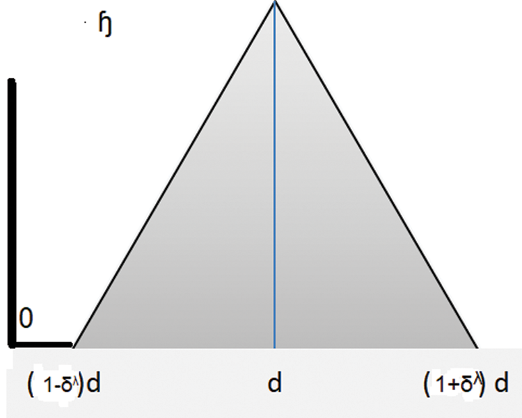
Figure 1:: The symmetric triangle fractal fuzzy value of Δtρ

where d indicates the shrinking middle point (a halfway point), Ldtρ:=(1−δd)d represents to the left side of d, and Rdtρ:=(1+δd)d indicates the right side of d.

δd denotes the spread function formulating as a variance function in terms of selling price (the impulse response point):

(for some constants a1 and a2 in R ). Moreover, the symbol η is equivalent to ηλ(d)≡(d,Ldtρ,Rdtρ) representing to the membership grade of the element d in the set Δtρ and is known as the membership function. By the definition of the spread function, we may describe any value in the above space as follows:

We proceed to define another item in the parametric space, which is the fuzzy buying cost, as follows:

B∁tȷ={(♭,ηλ(♭)):η(♭)=(♭,(1−δ♭)♭,1+δ♭)♭)}, (2)

where ♭ is the middle price of the type oil ȷ , L♭tȷ:=(1−δ♭)♭ is the left part of ♭ and R♭tȷ:=(1+δ♭)♭ is the right part to ♭ of the type oil ȷ at month t. Now, we introduce the uncertain production price as follows:

P∁t,φρ={(℘,η(℘)):η(℘)=(℘,(1−δ℘)℘,(1+δ℘)℘)}, (3)

where ℘ is the rough middle value, L℘t,φρ:=(1−δ℘)℘ is the left part of ℘ and R℘t,φρ:=(1+δ℘)℘ is the right part to ℘ of the type oil ρ at month t from refinery φ. Similarly, we define the rest of parametric spaces, fuzzy inventory price, fuzzy transportation and fuzzy management value, respectively as follows:

I∁t,φρ={(ι,ηλ(ι)):η(ι)=(ι,(1−δι)ι,(1+δι)ι)}, (4)

⊤∁t,φρ={(τ,ηλ(τ)):η(τ)=(τ,(1−δτ)τ,(1+δτ)τ)}, (5)

M∁t,φρ={(μ,ηλ(μ)):η(μ)=(μ,(1−δμ)μ,(1+δμ)μ)}. (6)

2.2 Local Fractional Difference Operator

Yang presented the local fractional derivative (fractal) of the function g(x) of order (0 < λ < 1) at the fixed value x0 as [10]:

υλg(x)=limx→x0Dλ(g(x)−g(x0))(x−x0)λ, (7)

where Dλ(g(x)−g(x0))≈Γ(λ+1)D(g(x)−g(x0)) and the forward difference D formulated as D(g(x)−g(x0))=g(x)−g(x0) , and Γ represents the gamma function Γ(n+1)=n!.

Now, by using the concept of a fractal, we introduce a generalization of the spread function δd(∁tρ)=a1+a2∁tρ as in the following fractal difference equation

δdλ(∁tρ):=Dλ(δd(∁tρ)−δd(∁0ρ))≈Γ(λ+1)D(δd(∁tρ)−a1)=Γ(λ+1)(δd(∁tρ)−a1)=a2Γ(λ+1)∁tρ,:=λΓ(λ+1)∁tρ, (8)

where a2=λ,δd(∁tρ)>0,δd(∁0ρ)=a1 and the fractal λ∈(0,1). Note that if λ∈(0,1), then we have Γ(λ+1)∈(0,1). In this place, we note that λ plays a critical role in improving the classical system when λ≈1 (see [11]). In our investigation, we suppose that λ=0.5 to get a good result for maximization. We shall use the fractal difference operator δdλ in all spaces given in Eqs. (1)–(6). For example, a fuzzy fractal demand Δtρ of the manufacture ρ at the month t becomes

Δtρ={(d,ηλ(d)):ηλ(d)=(d,(1−δdλ)d,(1+δdλ)d)tρ} (9)

where d indicates the shriveled middle point (i.e., halfway point), Ldtρ:=(1−δdλ)d represents to the left side of d and Rdtρ:=(1+δdλ)d indicates the right side of d . δdλ is given in Eq. (8). Similarly, for the other parametric spaces B∁tȷ,P∁t,φρ,I∁t,φρ,⊤∁t,φρ and M∁t,φρ .

3  Mathematical Modeling System

Under a fuzzy economic situation and constraints on manufacturing ability, inventory and operations, we propose a mathematical model to sustain a master buying and manufacturing proposal such that when the fluctuating demand is achieved, the maximum gain can be attained at an acceptable flat value.

3.1 Objective Function

The aim is to maximize the Πt which is formulated by

Maximize∑t‍(Πt−B_∁t−P_∁t−I_∁t−T_∁t−M_∁t), (10)

where χtȷ,Θφ,tρ,Iφ,tρ,Tφ,tρ are variables.

3.2 Constraint Inequalities

We have the following list of constraints inequalities:

• Invention of manufacturing in a month plus the previous manufacturing inventory must be larger than or equal to the fluctuating demand (variation demand) for the manufacturing. Therefore, we suggest the average by using λ as follows:

(1Φ∑φ?(Θφ,tρ+Iφ,t−1ρ)1/λ)λ≥(d,(1−δdλ)d,(1+δdλ)d)tρ, (11)

• The invention of every manufacturing at all refineries should be no less than the economical manufacture quantity of every manufacture at all refineries. Consequently, we obtain the following inequality

Θφ,tρ≥M_φ,tρ,(t=1,…,T,ρ=1,…,P,φ=1,…,Φ); (12)

• The manufacturing at all refineries is controlled by the maximum production capability. Thus, we conclude the following inequality

Θφ,tρ≤M_φ,tρ,(t=1,…,T,ρ=1,…,P,φ=1,…,Φ); (13)

• The quantity of every category of oil produced should be greater than or equal to the minimum monthly buying amount of every category of oil by agreements. Hence, we obtain the next inequality

χtȷ≥B_tȷ,(ȷ=1,…,J;t=1,…,T); (14)

• The total sum of oil purchases rendering to agreements is at least a positive fraction β (balance parameter) of the total sum of basic oils by the refinery manufacturing. Then as a conclusion, we have the constrained inequality

∑ȷ‍B_tȷ≥β∑ȷ‍χtȷ,,(ȷ=1,…,J;t=1,…,T); (15)

• The total of manufactured material transported from a refinery by any type of transportation (trains, pipelines or trucks) is less than or equal to the maximum permissible amount of the transportation

Tφ,tρ≤T_φ,tρ(t=1,…,T,ρ=1,…,P,φ=1,…,Φ); (16)

• The overall sum of manufactured material transported from refineries ought to be less than or equal to the refineries’ overall manufacturing output. Hence, we get the inequality

∑φ?Tφ,tρ≤∑φ?Θφ,tρ,(t=1,…,T,ρ=1,…,P,φ=1,…,Φ); (17)

• The overall sum of manufactured material transported from refineries has to be greater than or equal to the fluctuating (changing) demand for the manufacturing process. Connected to what has been mentioned above, we have the following constrain

∑φ?Tφ,tρ≥(d,(1−δdλ)d,(1+δdλ)d)tρ,t=1,…,T,λ∈(0,1),ρ=1,…,P,φ=1,…,Φ); (18)

• Overall, the variables must be non-negative

χtȷ,Θφ,tρ,Iφ,tρ,Tφ,tρ≥0,(ȷ=1,…,J,ρ=1,…,P;λ∈(0,1),t=1,…,T,φ=1,…,Φ). (19)

4  The Technique

The following steps represent our technique, respectively:

4.1 The Result of the Objective Function

We aim to maximize the objective function Λ=cχ, where c indicates symmetric coefficients. By utilizing the symmetric coefficient terms:

Based on the 3-D parametric space, we represent the objective function by the 3-multi-objective system, as follows:

maxΛ1=c1χ1+…+cnχnmaxΛ2=lλc1χ1+…+lλcnχnmaxΛ3=rλc1χ1+…+rλcnχn, (20)

where lλ=1−δcλ and rλ=1+δcλ. The next step is to compute the upper and lower bound of Λ, ( ΛU,ΛL ) . Accordingly, we have the following system for the lower bound

Λ1L=min(c1χ1+…+cnχn)Λ2L=min(lλc1χ1+…+lλcnχn)Λ3L=min(rλc1χ1+…+rλcnχn), (21)

and the following system for the upper bound

Λ1U=max(c1χ1+…+cnχn)Λ2U=max(lλc1χ1+…+lλcnχn)Λ3U=max(rλc1χ1+…+rλcnχn). (22)

Following the membership function of Λ, we employ:

ηλ(Λ)={0,Λ≤ΛLΛ−ΛLΛU−ΛL,ΛL<Λ≤ΛU1,Λ>ΛU (23)

where we aim to maximize ηλ(Λ); or maximize ⋎=min(⋎1,⋎2,⋎3) where ηλ(Λ)≥⋎. This solves the following issue:

max⋎,subjectto(c1χ1+…+cnχn)−⋎1(Λ1U−Λ1L)≥Λ1L(lλc1χ1+…+lλcnχn)−⋎2(Λ2U−Λ2L)≥Λ2L(rλc1χ1+…+rλcnχn)−⋎3(Λ3U−Λ3L)≥Λ3Lχi≥0,i=1,…,n⋎∈[0,1], (24)

where ΛkL,k=1,2,3 is given in Eq. (21).

4.2 Transportation Problem

We formulate the multiple objective functions (Λ1,Λ2,Λ3) based on Eq. (10) as follows:

maxΛ1=∑t‍(Πt−B∁t−P∁t−I∁t−T∁t−M∁t)maxΛ2=∑t‍(Πt−(1−δ∁λ)(B∁t+P∁t+I∁t+T∁t−M∁t))maxΛ3=∑t‍(Πt−(1+δ∁λ)(B∁t+P∁t+I∁t+T∁t−M∁t)), (25)

where δ∁=a1+a2∁,a1,a2∈R. Next, by utilizing Mathematica 11.2, we compute the upper and lower bounds. Accordingly, the system becomes as follows:

∑t‍(Πt−B∁t−P∁t−I∁t−T∁t−M∁t)−⋎1(Λ1U−Λ1L)≥Λ1L∑t‍(Πt−(1−δ∁λ)(B∁t+P∁t+I∁t+T∁t−M∁t))−⋎2(Λ1U−Λ1L)≥Λ2L∑t‍(Πt−(1+δ∁λ)(B∁t+P∁t+I∁t+T∁t−M∁t))−⋎3(Λ1U−Λ1L)≥Λ3L. (26)

Next, we proceed to convert the fuzzy inequality constraints as it is implied by Eqs. (11) and (18):

(1Φ∑φ‍(Θφ,tρ+Iφ,t−1ρ)1/λ)λ−⋎d(1−(1−δdλ))tρ≥d(1−δdλ)tρ,λ∈(0,1), (27)

and

∑φ‍Tφ,tρ−⋎d(1−(1−δdλ))tρ≥d(1−δdλ)tρ. (28)

Finally, we combine the multi-objective functions to maximize the following:

maxγ, subjectto∑t(Πt−B∁t−P∁t−I∁t−T∁t−M∁t)−γ1(Λ1U−Λ1L) ≥Λ1L∑t(Πt−(1−δ∁λ)(B∁t+P∁t+I∁t+T∁t−M∁t))−γ2(Λ1U−Λ1L) ≥Λ2L∑t(Πt−(1+δ∁λ)(B∁t+P∁t+I∁t+T∁t−M∁t))−γ3(Λ1U−Λ1L) ≥Λ3L(1Φ∑φ(Θφ,tρ+Iφ,t−1ρ)1/λ)λ−γ d(1−(1−δdλ))tρ ≥d(1−δdλ)tρ∑φTφ,tρ−γ d(1−(1−δdλ))tρ≥d(1−δdλ)tργ∈[0,1], (29)

taking in account that inequalities (12)-(17) and (19) are all achieved.

5  Document of the Development

We applied the above mentioned model in the Iraqi Patrol Company (IPC). IPC is the major oil manufacturing firm in Iraq. This company has one part located in Kirkuk city in northern Iraq, and another in Basrah city in southern Iraq. While there are four sub-companies in the middle of Iraq: Al-Doura, Al-Samawa, Al-Najaf and Al-Diwaniya (all have four yields) correspondingly. In this study, we dealt with the primary materials, specifically Gasoline (Ga), Kerosene (Tk), Gas oil (Go) and Fuel oil (Fo). The types of plain oils were limited to the four types mentioned above, and the planning and manufacturing period was set to T = 12 months (between 2018 and 2019).

To ensure an acceptable oil source, the IPC must come to an agreement with industrial oil countries. Relevant to our work, each group of basic oil j must be delivered in every month t . Fig. 2 depicts the stages of our procedure.

5.1 Data Analysis

To find the optimal solution, we collected our data as in Appendix A from its sources. Fig. 3 provides symmetric triangle values based on the parameter values 0<λ<1. The tables involve three values of λ:0.2,0.5,0.8; which implies three different values of ⋎ . It is evident that there is a relation between ⋎ and λ which can be recognized by the equation (Λ1,Λ2,Λ3) . Each product has its own parameter fuzzy value λ. For example, to determine (Λ1,Λ2,Λ3) for the production costs, we search for the maximum value in all refineries (which is 28.8 in the Al-Samawa refinery). Then by setting the three values λ:0.2,0.5,0.8, we determine the parametric fuzzy number of the product by using (8) as follows:

For λ=0.2 , we have λΓ(1+0.2)=0.2×0.91≈0.2→λ_=1−0.2=0.8 . Therefore, we obtain two parametric fuzzy numbers corresponding to 28.8:(23.04,51.84) (see Fig. 3). This new method provides many advantages, such as high accuracy and stability of the data. Using the information in Section 3 and Section 4, we follow the steps:

• Step 1: we obtained the upper bounds Λ3 and lower bounds Λ2 of the objective function (see the second and third column of the first matrix in Fig. 3, respectively)

• Step 2: we determine the vector (GaTkGoFo) by employing the values in step one. This vector represents the interval or the best value of ⋎; for instance, the value ⋎=0.5 implies the proper evaluation for the left and right amounts of the triangle.

• Step 3: Using the vector in step two, we estimate the interval or the value of ⋎∈[0,1] to maximize the problem in (24). As we realize that the value of ⋎=λ (the fractal parameter). Based on the analysis shown in Fig. 3, the most accurate analysis is given when λ=0.5.

• Step 4: By employing the vector in step two, we calculate the interval or the value of ⋎∈[0,1] to maximize the problem in (24). In this place, we confirm that by using Mathematica 11.2, solving system (24) implies that the exact value ⋎≈45 maximizes the system.

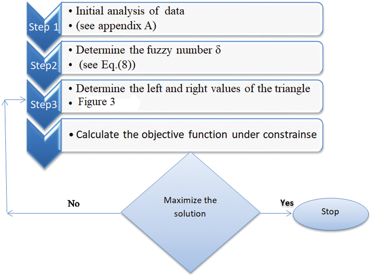
Figure 2:: Steps to maximize the solution and find the best interval of ϒ

5.2 Impact Analysis

Since the hypotheses and incomes are time irregular, several mathematical tests can describe the impact of uncertainty of the recent model. By shifting both demand and the price factors, as well as the estimate of the systems (see Fig. 3) with various symmetric triangular fuzzy number, the demand D and the price factors can be examined. The graphs in Fig. 3 indicate the date of the corresponding matrix (Λ1,Λ2,Λ3); The data show that the manufacturers’ order conferring to income action is unaffected by rises in the selling cost.

6  Discussion and Conclusion

We point out the following facts for our data that is collected in Appendix A.

• Modeling system: The fuzzy system can compute variables such as the selling and demand. This system has the ability to consider the relation between the selling amount and demand is investigated in three cases (real, upper and lower). The consequence limits the accumulative profit rule of gathering, buying amount, and selling value at the same average, while minimizing both at the same rate gives the least profit. The significance of a membership takes back to first principles of elastic and broader requests; it also provides a current systematic method with beneficial outcomes.

• Study case: This analysis illustrates that when there is more manufacturing yield, the total price will be lower, and vice versa. Nonetheless, the manufacturing design must trade-off demand and output, and the maximum market demand controls it. A study on IPC recognized uncertain market demand and different prices in the indefinite setting. The dynamics and outcomes indicate that the developed system is capable of delivering valuable data for increasing profit-effective oil refinery approaches under different settings.

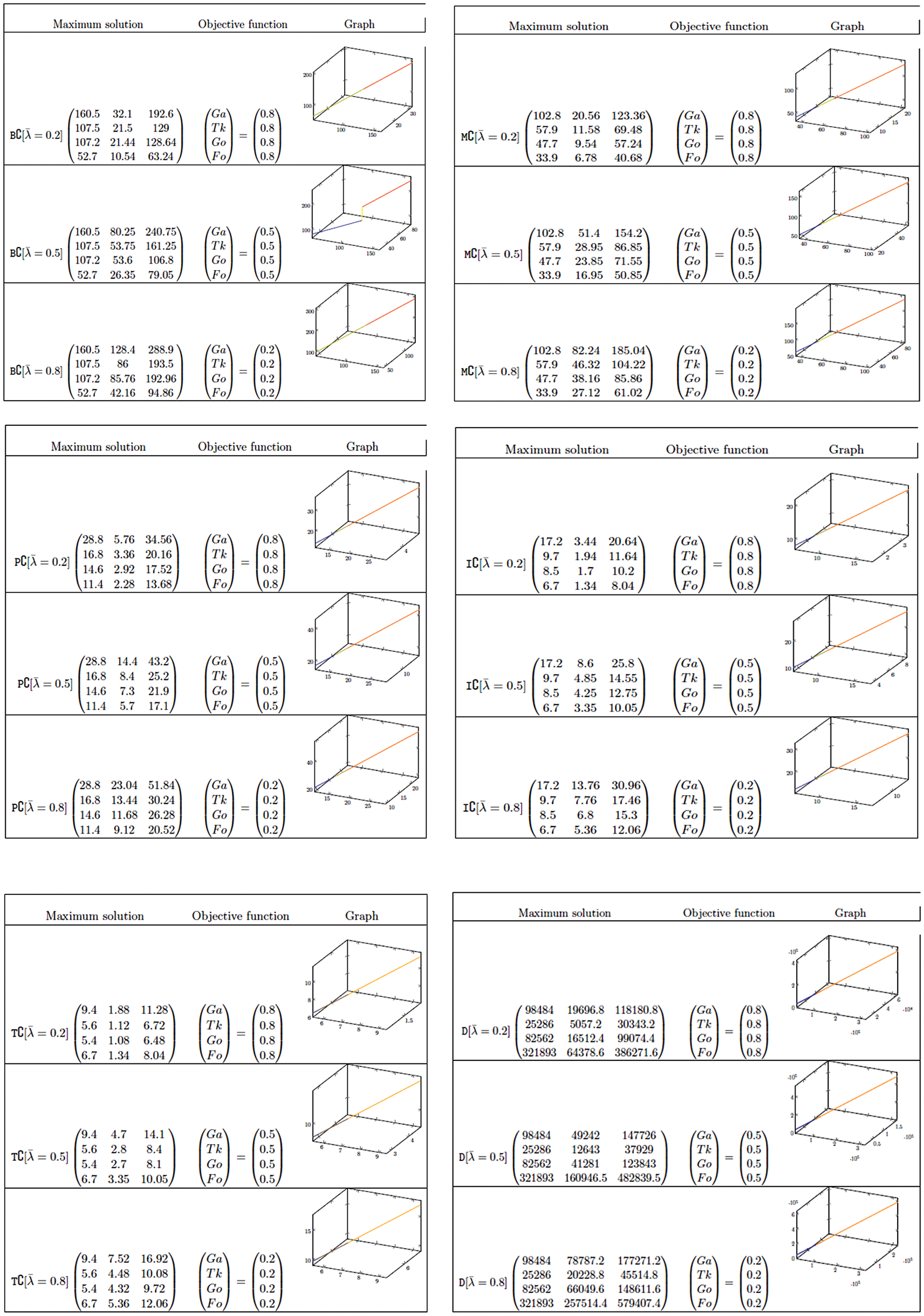
Figure 3:: From the top, Selling block costs, Management block costs, Product costs, Inventory costs, transportation costs and demand costs with λ_ = 0.2; 0.5; 0.8 respectively

Acknowledgement: The authors would like to express their thanks to the Iraqi Patrol Company to provide us with all the data under document number 783 in 2018-2019. The authors also would like to acknowledge Prince Sultan University for paying the Article Processing Charges (APC) of this publication. Finally, we would like to thank the editor and reviewers for their valuable comments.

Author Contributions: All authors have contributed to, read and agreed to the published version of the manuscript.

Availability of Data and Materials: Please contact authors for data requests.

Funding Statement: This research received no external funding.

Conflicts of Interest: The authors declare that they have no competing interests.

This work is licensed under a Creative Commons Attribution 4.0 International License, which permits unrestricted use, distribution, and reproduction in any medium, provided the original work is properly cited.