Intelligent Automation & Soft Computing DOI:10.32604/iasc.2021.018214
Article

Robust Optimal Proportional–Integral Controller for an Uncertain Unstable Delay System: Wind Process Application

Rihem Farkh1,2, Yasser Fouad1,* and Haykel Marouani1

1College of Engineering, Muzahimiyah Branch, King Saud University, Riyadh, 11451, Saudi Arabia
2Laboratory for Analysis, Conception and Control of Systems, LR-11-ES20, Department of Electrical Engineering, National Engineering School of Tunis, Tunis El Manar University, Tunis, 1002, Tunisia
*Corresponding Author: Yasser Fouad. Email: yfouad@ksu.edu.sa
Received: 01 March 2021; Accepted: 04 April 2021

Abstract: In industrial practice, certain processes are unstable, such as different types of reactors, distillation columns, and combustion systems. To ensure greater maneuverability and improve the speed of response command, certain systems in the military and aviation fields are purposely configured to be unstable. These systems are often more difficult to control than stable systems and are of particular interest to designers and control engineers. Despite all advances in process control over the past six decades, the proportional–integral–derivative (PID) controller is still the most common. The main reasons are the simplicity, robustness, and successful applications provided by PID-based control structures. The design of proportional–integral (PI) controller for time-delay (TD) systems is a traditional and classical problem. On one hand, PI controllers are used in more than 95% of industrial processes. On the other hand, there are TD phenomena in almost all practical control systems. In this paper, we study the robustness of a PI controller in stabilizing systems containing uncertain parameters and delays. A robust controller for an unknown unstable second-order with margin TD is constructed using a generalized Kharitonov theorem for quasi-polynomials. A constructive method based on the Hermite–Biehler theorem is used to obtain all PI gains, which stabilize an uncertain and unstable second-order delay system. Genetic algorithms (GAs) and optimization methods are used to obtain optimal system and control parameters for providing the best PI control that makes the system robust and stable under uncertainty. By minimizing performance criteria such as the integral of square error, integral of absolute error, time-weighted integral of absolute error, and integral of time weighted square error, GAs and particle swarm optimization are used to optimize the PI parameters and system parameters that provide the best control under uncertainties.

Keywords: Unstable time-delay system; interval plants; Generalized Kharitonov Theorem (GKT); PI controller; Hermite–Biehler theorem; stability region; genetic algorithms; Particle swarm optimization; optimum PI controller; optimum system parameters; wind process application

1  Introduction

Time delays are found in several industrial processes and engineering systems, such as hydraulic systems, turbojet engines, chemical processes and communication networks. Delays have a considerable effect on the dynamic behavior of closed-loop control systems and can cause oscillations and even lead to instability [1]. According to Gao et al. [2], over 90% of the physical systems in process control can be modelled by first-order + time-delay (TD) and second-order + TD (about 30%) models with tolerable accuracy.

Open-loop unstable delay systems are popular in the processing industry. Compared with stable open-loop systems, open-loop unstable delay systems pose a relatively challenging problem for controller design. In an unstable delay system, the presence of an unstable pole imposes a minimum control performance limit, which could yield long settling time and excessive overshoot.

Although the proportional–integral–derivative (PID) controller is an antiquated design, numerous applications for the control of industrial process prefer and widely use it. This is because of its simple structure, satisfactory control effect, and acceptable robustness [3]. Over the past six decades, numerous techniques have been used to calculate the parameters PID controller of systems with long TD. The use of PID controllers to stabilize uncertain systems with or without delay has received a lot of attention.

A generalization of the Hermite–Biehler theorem (HBT) is one of the well-known methods for determining the stabilizing PID controller region [4]. To define all stabilizing regions of PID parameters, this approach necessitates sweeping over the proportional gain. An extended theorem, which was used to locate the PID stabilizing parameter regions, used the HBT as its basis. Farkh et al. [5] have derived the complete stabilizing set of the classical proportional–integral (PI) and PID controller parameter regions for unstable second-order TD plants.

Ma et al. [6] presented explicit lower bounds on the delay margin of second-order unstable delay systems using PID controller. In Wang et al. [7], a multiple dominant pole placement for an unstable delay system, was used to build a PID controller with a lead/lag filter. An internal model control-PID controller was proposed for an unstable second-order TD system, which shows the characteristics of inverse response [8]. PID controller tuning using genetic algorithm (GA) for stable and unstable process was presented in Ayas et al. [9]. A particle swarm optimization (PSO) algorithm was proposed to tune and retune the parameter of PID controller for a class of unstable TD systems [10].

Over the last few decades, there has been a lot of interest in the stable stability of uncertain systems. For the stability analysis of interval systems, the Kharitonov theorem (KT) is well-known. The performance and stability of plants that are exposed to uncertainties are defined as robustness.

The edge theorem in Barmish et al. [11] and the box theorem in Kwon et al. [1] were based on KT and suggested that the set of transfer functions generated by varying its perturbed coefficients in the defined ranges corresponds to a box in the parameter space and is referred to as "interval plants."

Generalized KT (GKT) states that a controller robustly stabilizes an interval system if it stabilizes a specified set of line segments in the plant parameter space [12,13].

Researchers have expanded the GKT and edge theorem to determine the robust stability of a TD system subjected to parametric uncertainty in the case of quasi-polynomials [14,15].

Relevant results relating to the stabilization of interval systems have been acquired from previous studies. In Barmish et al. [16], it was proven that a first-order controller stabilized an interval plant if and only if the controller stabilized the 16 plants of the Kharitonov plant family at the same time.

A parameter plan based on KT and the gain phase margin tester method was used in Huang et al. [17] to obtain the nonconstructive region of a PID controller, which stabilizes the entire interval plants.

The stability boundary locus can be used to find the stabilizing region of PI parameters for the regulation of a plant with unknown parameters, according to Tan et al. [18].

Patre et al. [19] suggested a two-degrees-of-freedom design technique for interval process plants to ensure robust stability and satisfactory performance.

To stabilize a delay-free interval plant family, the HBT was employed in Refs. [20,21] to formulate the proportional, PI, and PID controllers. The stabilizing problem of a PI/PID controller was studied for a first-order delay system and then used to find both PI and PID gains that stabilize an interval first-order delay system [22].

We propose in this paper to extend the work presented in Farkh et al. [23] by determining the set of all PI gains that stabilize an unstable uncertain second-order delay system with coefficients that are perturbed within prescribed ranges. Applying GAs and PSO algorithms in the robust stable region using integral performance criteria, the optimal PI controller and optimal system parameters are then calculated.

2  Problem Formulation

A tool to design a robust PI controller for an unstable second-order system with bounded uncertain parameters and bounded uncertain TD is proposed in this paper.

We consider the plant family F(s)=Ke−Lss2+a1s+a0 , where K > 0, L > 0, a0 < 0, and a1 > 0 and K∈[K_,K¯] , a1∈[a1_,a1¯] , a0∈[a0_,a0¯] and L∈[L_,L¯] .

By combining robust stabilization results obtained earlier [4], which are presented in Section 5, and the approach developed in Section 3, we designed a robust PI controller that stabilizes the uncertain plant family F(s) . In Section 4, we show that stabilizing a plant family, where K∈[K_,K¯] , a1∈[a1_,a1¯] , a0∈[a0_,a0¯] , and L=L¯=Lmax , is enough to compute a robust stability region in the parametric space of the PI controller.

3  PI Controller Design for Unstable Second-Order Delay System

In Farkh et al. [5], all stabilizing PI controllers’ computation for an unstable delay system was considered.

3.1 Theorem 1 [5]

Under the assumptions, K > 0, L > 0, a0 < 0, and a1 > 0, the Kp values for which there is a solution for the stabilization problem of the PI controller of unstable second-order delay system, verify

where α is the solution of the equation below.

tan⁡(α)=α(2+a1L)(α2−a1L−a0L2) in the interval [0,π].

The range of Ki values is given by 0<Ki<Minj=1,3,5…⁡aj

where aj=a(zj)=zjKL[sin⁡(zj)(a0–zj2L2)+a1zjLcos⁡(zj)]

and zj,j=1,3,5,… are the roots, arranged in ascending order of magnitude, as follows.

3.2 Example

Consider the following transfer function for a second-order delay system:

To determine the values of Kp , we search for α in interval [0,π] satisfying: tan⁡(α)=4.5α(α2−2.625)⇒α=1.5617 .

For Kp , the range is given by 0.25<Kp<7.85 .

We notice that

Consequently, we choose the final range of Kp as 0.25 < Kp < 6.2

The system stability region is obtained in (Kp,Ki) ; Fig. 1 presents the plane.

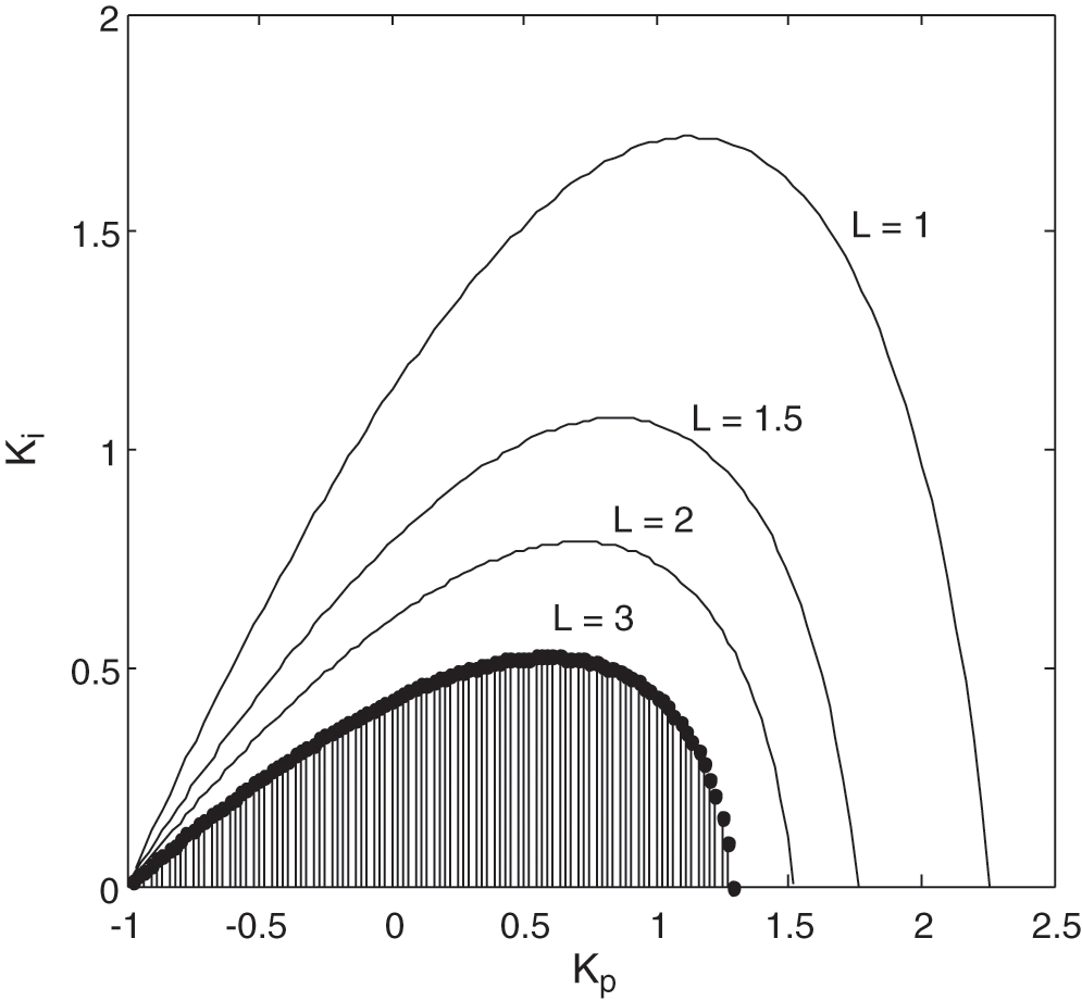
Figure 1: Sets of stabilizing PI controllers for Example 1

4  Design of a Robust Controller for an Unstable System with an Uncertain Delay

The problem of stabilizing an unstable second-order system with TD is presented in this section., where the parameters K , a1, and a0 are known and the TD is unknown but lies inside a known interval.

We consider the following plant family: F1(s)=Ke−Lss2+a1s+a0 , where L∈[L_,L¯] , K , a1, and a0 are known.

4.1 Lemma 1 [4]

Consider the system with a transfer function F1(s) . If a given PI controller stabilizes the delay-free system and the system L=L¯>0 , then the same PI controller stabilizes the system ∀L∈[0,L¯] .

4.2 Example

Consider the plant family F1(s)=1.9e−Lss2+4s−0.4 , where L∈[0.1,0.5] seconds. The set of all stabilizing PI controllers for different TD values can be found using the algorithm presented in Farkh et al. [5].

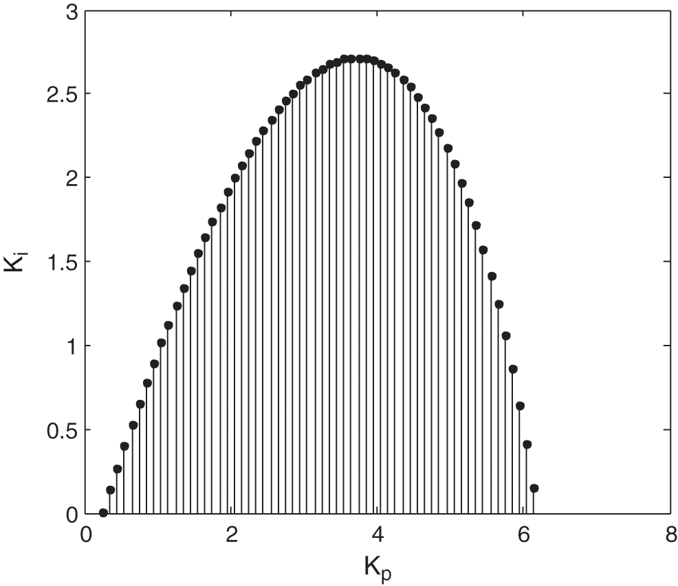
Figure 2: (Kp,Ki) Controller stability region for unstable second-order delay system

Fig. 2 represents these sets for L=1,1.5,2,3 . The intersection of all these sets is the set corresponding to L = 3 (dashed area).

Thus, any PI controller from this set will stabilize the entire family of plants described by F1(s) . In view of Lemma 1 because the closed-loop system is stable for L¯ , it is also stable for L∈[L_,L¯] .

This result is used to simplify the problem stabilization of the family plant F(s) to design a robust controller such that the following parameters verify K∈[K_,K¯] , a1∈[a1_,a1¯] , a0∈[a0_,a0¯] , and L=L¯ .

The delay is set to L¯ for the rest of this article, which is the established upper bound of the TD.

5  Robust Controller Design for Interval System with Fixed TD

The procedure for finding a robust stabilization of an unstable delay system belonging to a linear interval plant is discussed in this section, where the TD, L, is a known constant.

Consider the transfer function below:

F(s)=F1(s)F2(s)e−Ls (1)

where F1(s) and F2(s) are linear interval polynomials. Our goal is to find a robust controller C(s)=C1(s)C2(s) with fixed polynomials C1(s) and C2(s) to guarantee the system’s robust stability.

To compute all the stabilizing controller parameters for interval systems with TDs, we can use the GKT expanded for quasi-polynomials [13]. Before stating the GKT, we study some results from the field of robust parametric control.

Consider the following family of quasi-polynomials Δ(s) :

Δ(s)=F1(s)C1(s)+F2(s)C2(s) (2)

− F_(s)=(F1(s),F2(s)) is a fixed two-tuple of real interval polynomials, where each Fi(s) is a linear interval polynomial characterized by the intervals Fj,i as follows:

Fj,i∈[F_j,i,F¯j,i],i=1,2;j=0,1,…,ni. (3)

Fi(s) is a real independent interval polynomial described as:

Fi(s)=f0,i+f1,is+…+fni,isni,i=1,2. (4)

− C_(s)=(C1(s),C2(s)) is a fixed two-tuple of complex quasi-polynomials in the following form:

Ci(s)=Ci0(s)+Ci1(s)e−sLi1+Ci2(s)e−sLi2+… (5)

where Cij(s) are complex polynomials satisfying the following condition:

degree[Ci0(s)]>degree[Cij(s)],j≠0 (6)

In this sudy, we use Ci(s) with a single delay as: Ci(s)=Ci0(s)+Ci1(s)e−sLi .

The stability problem (2) can be solved with the GKT by constructing an extremal set of line segments ΔE(s)⊂Δ(s) , where the stability of ΔE(s) implies the stability of Δ(s) , according to Bhattacharyya et al. [2].

ΔE(s) will be produced by constructing an extremal subset FE(s) , which is derived from the Kharitonov polynomials of Fi(s) .

5.1 Theorem 2 [13]

Let C_=(C1(s),C2(s)) be a two-tuple of complex quasi-polynomials verifying condition (6) above, and let F_=(F1(s),F2(s)) be a polynomial with independent real intervals : the entire family F_(s) is stabilized C_(s) if and only if C_ stabilizes every two-tuple segment in FE(s) . Equivalently, Δ(s) is stable if and only if ΔE(s) is stable.

5.2 Corollary

The linear system F_(s) is stabilized by C_(s) , if and only if the controller stabilizes the extremal transfer function FE(s) . This is discussed in detail later.

To use the GKT, we must first define the most extremal set of line segments ΔE(s) . Eight Kharitonov vertex equations are derived from the segment polynomials of F1(s) and F2(s) .They are expressed by Refs. [13,15]:

and

where:

Ki1(s)=f_i,0+fi,1_s+fi,2¯s2+f¯i,3s3+…Ki2(s)=f_i,0+fi,1¯s+fi,2¯s2+f_i,3s3+…Ki3(s)=f¯i,0+f_1s+f_i,2s2+fi,3¯s3+…Ki4(s)=fi,0+fi,1¯s+f_i,2s2+f_i,3s3+… (7)

The extremal subset FEi(s),i=1,2, consists of:

FE1(s)=λK1l(s)+(1−λ)K1k(s)K2h(s)FE2(s)=K1h(s)λK2l(s)+(1−λ)K2k(s) (8)

where λ∈[0,1] , h=1,2,3,4 and [l,k] = [1,2] [1,3] [2,4] [3,4].

The number of extremal equations is (i4i) , where i denotes the number of perturbed polynomials and [l,k] present the connection points to make Kharitonov polytope λKil(s)+(1−λ)Kik(s) .

Some of the subset equations may be the same; hence, the extremal subset is described as [13]:

FE(s)=FE1(s)∪FE2(s) (9)

The extremal subset of line segments (or generalized Kharitonov segment polynomials) is [2]:

ΔE(s)=ΔE1(s)∪ΔE2(s)={<C(s),F(s)>:F(s)∈FE(s)} (10)

where

<C(s),F(s)>=C1(s)F1(s)+C2(s)F2(s)+…+Cm(s)Fm(s) (11)

With the knowledge that ΔE(s)⊂Δ(s) , If the linear interval system's polynomials are all stable, the system with perturbed parameters would be as well.

The robust parametric approach control technique is an efficient control design technique, as shown by the previous findings.

For the synthesis of controllers that simultaneously stabilize a given uncertain TD system, the following will be used.

6  Robust Stabilization for Uncertain Unstable Second-Order Delay System

The problem of characterizing all PI controllers that stabilize an unstable second-order interval plant with TD is addressed in this section.

F(s)=Ke−Lsa0+a1s+s2 , where K∈[K_,K¯] , a0∈[a0_,a0¯] , a1∈[a1_,a1¯] and fixed TD, L.

The controller is given by:

Using the GKT for quasi-polynomials, we can obtain all PI gains that stabilize F(s) , we will use the new transfer function F(s) as: F(s)=F1(s)F2(s)=Ke−Lsa0+a1s+s2 and the new compensator as follows:

The family of closed-loop characteristic quasi-polynomials Δ(s,Kp,Ki) becomes

Δ(s,Kp,Ki)=C1(s)F1(s)+C2(s)F2(s)=K(Ki+Kps)e−Ls+(a0+a1s+s2)s (12)

The problem of determining all stabilizing PI controllers is to find all the values of Kp and Ki for which the entire family of closed-loop characteristic quasi-polynomials is stable.

Let K1j(s) and K2j(s),j=1,2,3,4 be the Kharitonov polynomials corresponding to F1(s)=K and F2(s)=a0+a1s+s2 , respectively.

where: K∈[K_,K¯] , a0∈[a0_,a0¯] , and a1∈[a1_,a1¯] .

Let FE(s,λ) denote the family of 32 plant segments:

FE(s,λ)={Flkh(s,λ)/Flkh(s,λ)=λK1l(s)+(1−λ)K1k(s)K2h(s)∪Flkh(s,λ)=K1h(s)λK2l(s)+(1−λ)K2k(s)λ∈[0,1];h=1,2,3,4;[l,k]=[1,2],[1,3],[2,4],[3,4]} (13)

Then, FE(s,λ) it consists of the following plant segments, where the 32 extremal plants in Eq. (13) are reduced to 20:

FE(s,λ)={F1=K_a0_+a1_s+s2,F2=K_a0_+a1¯s+s2F3=K_a0¯+a1_s+s2,F4=K_a0¯+a1¯s+s2F5=K¯a0_+a1_s+s2,F6=K¯a0_+a1¯s+s2F7=K¯a0¯+a1_s+s2,F8=K¯a0¯+a1¯s+s2F9=K¯−λ(K¯−K_)a0_+a1_s+s2,F10=K¯−λ(K¯−K_)a0_+a1¯s+s2F11=K¯−λ(K¯−K_)a0¯+a1_s+s2,F12=K¯−λ(K¯−K_)a0¯+a1¯s+s2∪F13=K_a0_+(a1¯−λ(a1¯−a1_))s+s2,F14=K¯a0_+(a1¯−λ(a1¯−a1_))s+s2F15=K_a0_+λ(a0¯−a0_)+a1_s+s2,F16=K¯a0_+λ(a0¯−a0_)+a1_s+s2F17=K_a0_+λ(a0¯−a1_)+a1¯s+s2,F18=K¯a0_+λ(a0¯−a1_)+a1¯s+s2,F19=F4=K_a0¯+a1¯s+s2,F20=F8=K¯a0¯+a1¯s+s2λ∈[0,1]} (14)

The closed-loop characteristic quasi-polynomials for each of these 32 plant segments Flkh(s,λ) are denoted by δlkh(s,Kp,Ki,λ) and are defined as:

δlkh(s,λ)=sNum(Flkh(s,λ))+(Ki+Kps)den(Flkh(s,λ)) (15)

where:

{Num(Flkh(s,λ))=λK1l(s)+(1−λ)K1k(s)∪K1h(s)den(Flkh(s,λ))=K2h(s)∪λK2l(s)+(1−λ)K2k(s) (16)

We posit the following theorem on using a PI controller to stabilize a second-order interval plant with TD.

6.1 Theorem 3

Let F(s) be an unstable second-order interval system with uncertain TD; a PI controller stabilizes the entire family F(s) if and only if each Flkh(s,λ)∈FE(s,λ) is stabilized by the same PI controller.

6.2 Proof

According to Theorem 3, the entire family Δ(s,Kp,Ki) is stable if and only if δlkh(s,Kp,Ki,λ) are all stable. Therefore, a PI controller will stabilize the entire family F(s) if and only if every element of FE(s,λ) is simultaneously stabilized by the same PI controller.

To obtain the all PI controllers that stabilize the interval plant F(s) by applying this method to each Flkh(s,λ) belonging FE(s,λ) , we use the results in Farkh et al. [5].

6.3 Example

We consider the plant family F(s)=Ke−Lsa0+a1s+s2 where K∈[1.9,2.2] , a0∈[−0.6,−0.4] , a1∈[4,6] and L∈[0.1,0.5] .

The entire family FE(s,λ) is given as follows:

FE(s,λ)={Fij(s,λ)/F(s,λ)=λlK1l(s)+(1−λl)K1k(s)K2h(s)∪F(s,λ)=K1h(s)λmK2l(s)+(1−λm)K2k(s)λ∈[0,1];h=1,2,3,4;[l,k]=[1,2],[1,3],[2,4],[3,4]} (17)

According to Eq. (14), we obtain

FE(s,λ)={F1=1.9−0.6+4s+s2,F2=1.9−0.6+6s+s2F3=1.9−0.4+4s+s2,F4=1.9−0.4+6s+s2F5=2.2−0.6+4s+s2,F6=2.2−0.6+6s+s2F7=2.2−0.4+4s+s2,F8=2.2−0.4+6s+s2F9=2.2−0.3λ−0.6+4s+s2,F10=2.2−0.3λ−0.6+6s+s2F11=2.2−0.3λ−0.4+4s+s2,F12=2.2−0.3λ−0.4+6s+s2∪F13=1.9−0.6+(6−2λ)s+s2,F14=2.2−0.6+(6−2λ)s+s2F15=1.9−0.4+0.2λ+4s+s2,F16=2.2−0.4+0.2λ+4s+s2F17=1.9−0.4+0.2λ+6s+s2,F18=2.2−0.4+0.2λ+6s+s2,F19=G4=1.9−0.4+6s+s2,F20=F8=2.2−0.6+6s+s2λ∈[0,1]} (18)

We remark that from F9 to F18 , we have an infinity of transfer function’s sets due to their dependence on λ . To reduce this problem’s complexity, we set λ to 0, 0.33, 0.66, and 1 as different values of λ∈[0,1] for F9 to F12 .

We set λ to 0, 0.25, 0.5, 0.75, and 1 as different values of λ∈[0,1] for F13 to F18 .

Therefore, we obtain

{Fh_1=Fh1(s,λ=0)Fh_2=Fh(s,λ=0.33)Fh_3=Fh(s,λ=0.66)Fh_4=Fh(s,λ=1) (19)

We define Fk_p=Fh(s,λp) , where λp∈{0,0.25,0.5,0.75,1} for k=13,..,18 and p=1,…,5 .

We obtain

{Fh_1=Fh1(s,λ=0)Fh_2=Fh(s,λ=0.25)Fh_3=Fh(s,λ=0.5)Fh_4=Fh(s,λ=0.75)Fh_5=Fh(s,λ=0.75) (20)

The following figure (Fig. 3) presents the stabilizing (Kp,Ki) values for the entire family F(s) by invoking the result presented in Farkh et al. [5], which applies to each transfer function belonging to FE(s,λ) .

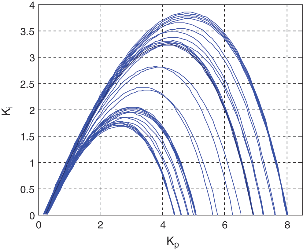
Figure 3: The stabilizing set of (Kp,Ki) for F(s)

An overlapped area of the boundaries is the intersection of these stability regions, which constitutes the entire feasible controller sets that stabilize the entire family F(s) (Fig. 4).

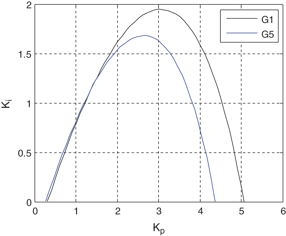
Figure 4: Final stability region in (Kp,Ki) the plan for interval plant

7  Optimization Controller Design

7.1 GAs optimization

GAs are effective stochastic search methods based on natural selection and evolutionary genetics principles.

GAs sustain a community of individuals. Individuals are adapted to a particular setting by changing the discovery, crossover, and mutation periods. People benefit from the environment's valuable knowledge (fitness), and the selection mechanism ensures that people of higher quality are preserved.

As a result, the population's overall output increases during the development cycle, ideally contributing to an optimal solution [24]. Because of its strong capacity for global optimization, GA is used in a variety of fields.

7.2 PSO

Particle swarm optimization (PSO) [25] is an artificial intelligence-based technique for maximizing and minimizing problems.

It was inspired by the social behavior of animals, such as birds flocking and fish schooling. It starts with a random set of solutions (known as particles). Each particle has its positions (value of variables) and velocities. It improves the initial solutions by updating velocities and positions.

Fig. 5 illustrates the theory of PSO and GA optimization for control problems.

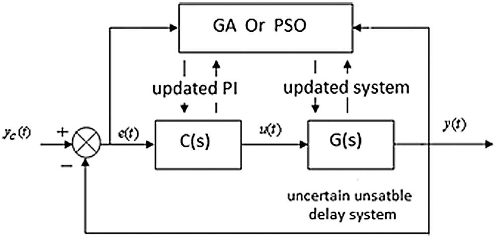
Figure 5: Optimization of controller and system parameters

In this case, it's in our best interests to find the best system and controller parameters in the robust stability area by combining one or more of the following criteria:, ISE,IAE,ITAE and ITSE defined by the following relationships:

7.3 Example

We consider the uncertain, unstable delay system F(s)=Ke−Lsa0+a1s+s2 where K∈[1.9,2.2] , a0∈[−0.6,−0.4] , a1∈[4,6] and L∈[0.1,0.5] .

The robust PI stability region is given in Fig. 4, from which Kp they Ki are choosing between Kp∈[0.2727,5.974] and Ki∈[0,1.9] .

The following table presents the optimum PI and system parameters supplied by GA and PSO.

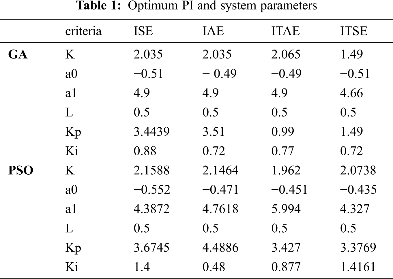
Using the values in Tab. 1, Figs. 6 and 7 show the closed-loop system's step responses.

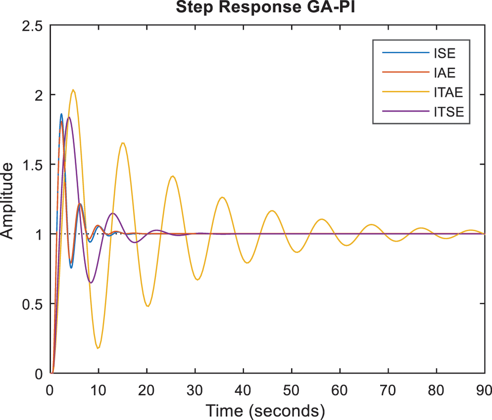
Figure 6: Step responses with GA-PI controllers

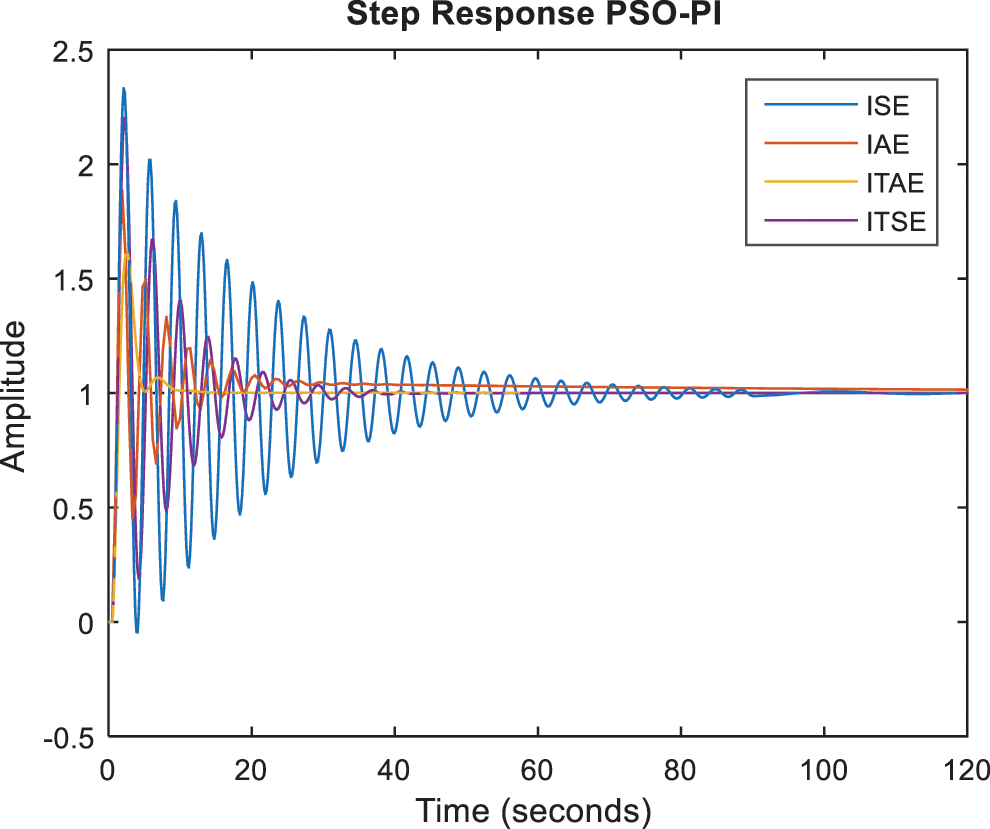
Figure 7: Step responses with PSO-PI controllers

The time parameter specifications are given in Tab. 2.

8  Conclusions

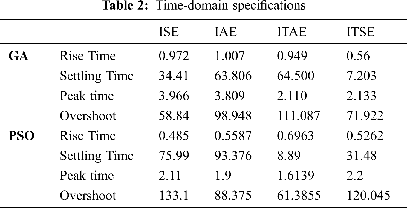
The HBT and GKT can be applied promptly to define the robust PI stability area for the control of uncertain and unstable second-order TD systems. The optimal system and optimal PI control parameters were computed using the integral performance criterion based on the optimization process's error.

Acknowledgement: The authors extend their appreciation to the Deputyship for Research and Innovation, Ministry of Education in Saudi Arabia, for funding this research work through the project number (DRI-KSU-1410)

Funding Statement: The authors received no specific funding for this study.

Conflicts of Interest: The authors declare that they have no conflicts of interest to report regarding the present study.

References

 1.  W. H. Kwon and P. G. Park, “Stability of time-delay systems,” in Communications and Control Engineering, Berlin, Springer, 2019. [Google Scholar]

 2.  Q. Gao and H. R. Karimi, Stability, Control and Application of Time Delay Systems. Butterworth-Heinemann, 1st edition, pp. 54–98, 2019. [Google Scholar]

 3.  C. Knospe, “PID control,” in IEEE Control Systems Magazine, vol. 26, no. 1, pp. 30–31, 2006. [Google Scholar]

 4.  G. J. Silva, A. Datta and S. P. Bhattacharyya, PID controllers for time delay systems. Springer, Berlin, 2005. [Google Scholar]

 5.  R. Farkh, K. Laabidi and M. Ksouri, “Stabilizing sets of PI/PID controllers for unstable second order delay system,” International Journal of Automation and Computing, vol. 11, no. 2, pp. 210–222, 2014. [Google Scholar]

 6.  D. Ma, J. Chen, A. Liu, J. Chen and S. I. Niculescu, “Explicit bounds for guaranteed stabilization by PID control of second-order unstable delay systems,” Automatica, vol. 100, pp. 407–411, 2019. [Google Scholar]

 7.  Z. Wang, X. Ran, B. Zhao and J. Zhao, “GA tuning PID controller based on second-order time-delay industrial system,” in MATEC Web of Conferences, vol. 288, 2019. [Google Scholar]

 8.  M. Kumar, D. Prasad and R. S. Singh, “Performance enhancement of IMC-PID controller design for stable and unstable second-order time delay processes,” Journal of Central South University, vol. 27, no. 1, pp. 88–100, 2020. [Google Scholar]

 9.  M. S. Ayas and E. Sahin, “Parameter effect analysis of particle swarm optimization algorithm in PID controller design,” An International Journal of Optimization and Control: Theories & Applications, vol. 9, no. 2, pp. 165–175, 2019. [Google Scholar]

10. V. Rajinikanth and K. Latha, “Tuning and retuning of PID controller for unstable systems using evolutionary algorithm,” ISRN Chemical Engineering, vol. 2012, pp. 1–10, 2012. [Google Scholar]

11. B. R. Barmish, C. V. Holot, F. J. Kraus and R. Tempo, “Extreme points results for robust stabilization of interval plants with first order compensators,” IEEE Transaction on Automatic Control, vol. 37, no. 6, pp. 707–714, 1992. [Google Scholar]

12. S. P. Bhattacharyya, H. Chapellat and L. H. Keel, Robust Control the Parametric Approach. Upper Saddle River, NJ: Prentice-Hall, 1995. [Google Scholar]

13. S. P. Bhattacharyya and H. Chapellat, “A generalization of Kharitonov's theorem: Robust stability interval plants,” IEEE Transaction on Automatic Control, vol. 3, pp. 306–311, 1989. [Google Scholar]

14. K. Gu and V. Kharitonov, “Robust stability of time-delay systems,” IEEE Transaction on Automatic Control, vol. 39, no. 12, pp. 2388–2397, 1994. [Google Scholar]

15. V. L. Kharitonov, J. A. Torres-Muñoz and M. B. Ortiz-Moctezuma, “Polytopic families of quasi-polynomials: Vertex-type stability conditions,” IEEE Transaction on Circuits and Systems, vol. 50, no. 11, pp. 1413–1420, 2003. [Google Scholar]

16. B. R. Barmish, C. V. Holot, F. J. Kraus and R. Tempo, “Extreme points results for robust stabilization of interval plants with first order compensators,” IEEE Transaction on Automatic Control, vol. 37, no. 6, pp. 707–714, 1992. [Google Scholar]

17. Y. J. Huang and Y. J. Wang, “Robust PID tuning strategy for uncertain plants based on the Kharitonov theorem,” ISA Transaction, vol. 39, pp. 419–431, 2000. [Google Scholar]

18. N. Tan, I. Kaya, C. Yeroglu and D. P. Atherton, “Computation of stabilizing PI and PID controllers using the stability boundary locus,” Energy Conversion and Management, vol. 47, pp. 3045–3058, 2006. [Google Scholar]

19. B. M. Patre and P. J. Deore, “Robust stability and performance for interval process plants,” ISA Transactions, vol. 46, pp. 343–349, 2007. [Google Scholar]

20. M. T. Ho, A. Datta and S. P. Bhattacharyya, “Design of P, PI and PID controllers for interval plants,” in Proc. of the American Control Conf., Philadelphia, PA, USA, vol. 4, pp. 2496–2501, 1998. [Google Scholar]

21. G. J. Silva, A. Datta and S. P. Bhattacharyya, “Robust control design using PID controller,” in Proc. 41 st IEEE Conf. on Decision and Control, Las Vegas, NV, USA, vol. 2, pp. 1313–1318, 2002. [Google Scholar]

22. R. Farkh, K. Laabidi and M. Ksouri, “Robust PI/PID controller for interval first order system with time delay,” International Journal of Modelling Identification and Control, vol. 13, no. 1/2, pp. 307–321,2011. [Google Scholar]

23. R. Farkh, K. A. Aljaloud, M. Ksouri and F. Bouani, “Optimal robust control for unstable delay system,” Computer Systems Science and Engineering, vol. 36, no. 2, pp. 307–321, 2021. [Google Scholar]

24. T. Jili, Z. Ridong and Z. Yong, “DNA computing based genetic algorithm,” in Applications in Industrial Process Modeling and Control. Springer, Berlin, pp. 25–55,2020. [Google Scholar]

25. A. Slowik, Swarm Intelligence Algorithms. CRC Press, United States, 2020. [Google Scholar]

This work is licensed under a Creative Commons Attribution 4.0 International License, which permits unrestricted use, distribution, and reproduction in any medium, provided the original work is properly cited.