DOI:10.32604/iasc.2021.019101
| Intelligent Automation & Soft Computing DOI:10.32604/iasc.2021.019101 | |
| Article |
A Two-Step Approach for Improving Sentiment Classification Accuracy
1Department of Computer Science & Information Technology, The Superior College Lahore, Lahore, 54000, Pakistan
2Department of Computer Science, The University of Lahore, Lahore, 54000, Pakistan
3Department of Electrical Engineering, Government College University, Lahore, 54000, Pakistan
4Department of Electrical Engineering, The Superior College Lahore, Lahore, 54000, Pakistan
*Corresponding Author: Rao Muhammad Asif. Email: rao.m.asif@superior.edu.pk
Received: 02 April 2021; Accepted: 17 May 2021
Abstract: Sentiment analysis is a method for assessing an individual’s thought, opinion, feeling, mentality, and conviction about a specific subject on indicated theme, idea, or product. The point could be a business association, a news article, a research paper, or an online item, etc. Opinions are generally divided into three groups of positive, negative, and unbiased. The way toward investigating different opinions and gathering them in every one of these categories is known as Sentiment Analysis. The enormously growing sentiment data on the web especially social media can be a big source of information. The processing of this unstructured data is of deep interest for researchers in the field of data science. The proposed article is an effort to find a model which can improve the classification accuracy of sentiment data. In this paper, a complete model is introduced to improve the accuracy of binary-class sentiment data. The model is reliable as it has been validated on three distinctive datasets with various sample sizes. In this regard, Amazon reviews, Yelp reviews, and IMDB reviews are taken into account. This model is based on completely referenced datasets and considerable improvement in accuracy is seen as compared to individual classifiers. Various heterogeneous classifiers are trained on the above-mentioned datasets at the base level. These base-level classifiers ought to be chosen from various groups of classifiers. At that point, the output of these base-level classifiers is consolidated to create a new dataset that acts as input for meta-level classifiers. At the meta-level, the base-level classifier with the best outcomes is selected with the new dataset framed. The model accordingly framed can be used to predict any sample query.
Keywords: Machine learning; classification; sentiment data; ensembles; heterogeneous ensemble; base learners
A lot of data has been added and moved between different electronic devices. One can't oversee a particularly massive measure of data physically, even our capacity to analyze the data slacks the ability to store, recover, and transfer it. The task of text classification has become a challenge when dealing with largescale printed data and fetching the required information.
According to an article published in c-sharpcornor.com “How much data on Internet”, the following are a few details of rapidly growing data on the Internet.
90% of Internet data is created in the last two years. Today, Internet hosts have around 2 billion active websites. There are 4.2 billion active users connected to the Internet all the time via 50 billion devices as shown in Fig. 1.
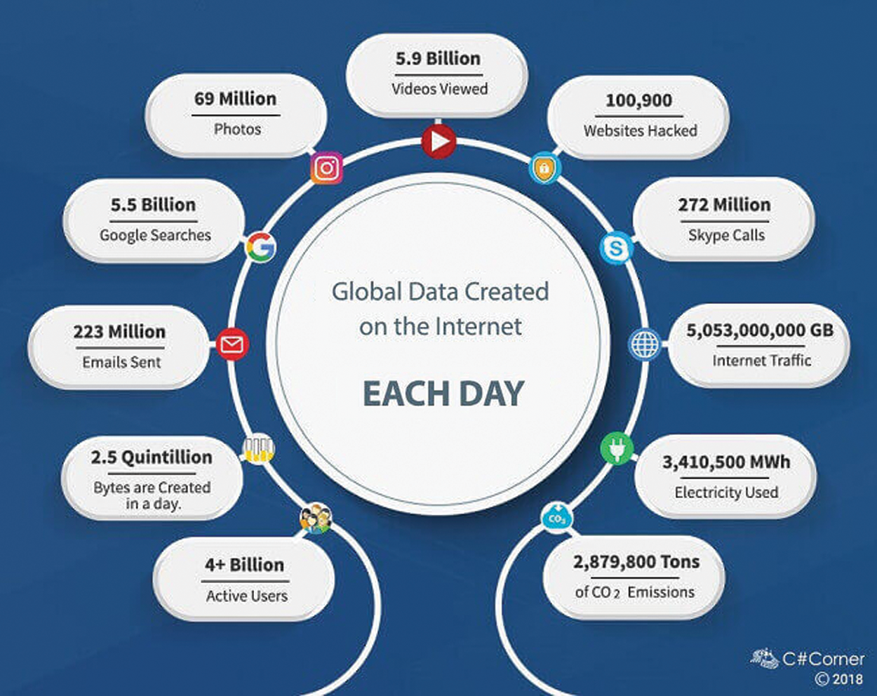
Figure 1: Internet live stats
Here are some daily numbers according to Internet Live Stats:
• 4+ billion active users
• 2.5 quintillion bytes created
• 223 million emails sent (the majority of them are spam emails)
• 5.5 billion Google searches
• 5.9 billion videos viewed on YouTube
• 69 million photos uploaded to Instagram
• 272 million Skype calls
• 100,900 websites hacked
• 5,053,000,000 GB Internet traffic
The major chunk of this data is unstructured, i.e., data is in the form of text, images, audio, or videos, etc.
As mentioned earlier, the job of classification is to deal with an enormous scope of textual data efficiently and extract required information quickly. With the extended need for data analysis for enormous data, there is a need for improvement of the performance of data mining and machine learning algorithms. Text classification organizes the constituent records depending on words, expressions, and phrases relating to a set of predefined classifications. There are various applications of text classification, for instance, extortion recognition, research paper ordering, item correlations, spam mail detection, research paper classification, content plan, and news arrangement.
Keywords contain the words that ultimately contain the most significant amount of information about text data. These keywords are then prepared to group a document. Similar examinations of substance classifiers have been conducted by various investigators. An examination of standard substance classifiers exhibits that a couple of classifiers produce extraordinary outcomes when there are just two classes. Nonetheless, when applied to multi-class textual data, their results are not satisfactory. This energizes the advancement of multi-class classifiers; Researchers can't discover a classifier or blend of classifiers that perform reliably well in all circumstances. The fundamental issue is which blend or kind of mix can be an outperformer. A large amount of text data is being moved to electronic devices consistently. Also, this data can be confined to different kinds of subspaces. An individual classifier may be a better classifier for some particular subspaces, but it may not be suitable for others. So, there is a need for a blend of classifiers that can yield better outcomes on the majority of these subspaces.
A novel blend of classifiers is introduced in this study for the improvement in the accuracy of classification systems. The core of the proposed methodology is to stack two or more classification algorithms for classification.
The purpose of this work is to present an improved hybrid classification model in R to classify or categorize textual data at the level of an individual publication.
Objectives:
Three main areas are under discussion in this paper.
1. Data representation. Since data is in raw form when extracted from the Internet, the first objective is to convert this informal data to formal representation by using several preprocessing steps.
2. Comparison of results of distinct base-level classifiers. At the base level, different machine learning classifiers are applied to check the individual performance. The next objective is a comprehensive comparison of the performance of base-level classifiers from different families.
3. Development of heterogeneous ensemble system. The last objective is to build a heterogeneous model by combining the output of base-level classifiers. The heterogeneous ensemble approach is supposed to work well to develop a hybrid machine learning system.
Modeling sentiments of human activities and opinions are becoming a striking research area, and awareness stays growing about its high-tech, analytical and social, and economic challenges [1]. Analysis and modeling of human sentiments can be established for several applications such as robotics [2], business decision making, tracking [3], skill assessments, sports, etc. [4].
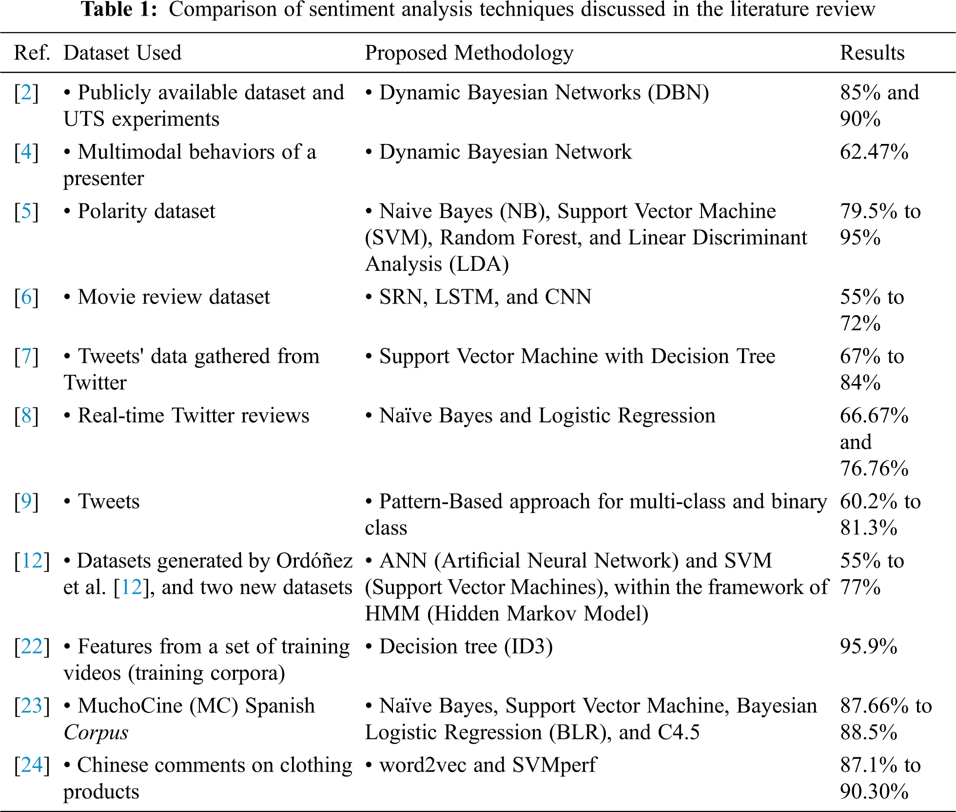
Different classification techniques are used by different researchers to obtain better accuracy. Different polarity groups can be constructed based on sentiment data for classification purposes. Four machine learning algorithms, viz. Naive Bayes (NB), Support Vector Machine (SVM), Random Forest, and Linear Discriminant Analysis (LDA), are considered in this paper for classification [5]. Besides, researchers explore the impact of two influential textual features, namely the word count and review readability, to evaluate the performance of SRN, LSTM, and CNN on a benchmark movie reviews dataset. Multiple regression models are further employed for statistical analysis. Their findings show better accuracy and reliability [6]. Ensemble learning strategies are used by other researchers in search of better accuracy. They find improved results by merging Support Vector Machine with Decision Tree, and experimental results prove that their proposed approach provides better classification results in terms of F-measure and accuracy in contrast to individual classifiers [7]. In this regard, the authors show that individual classifiers can also perform well. Prabhat et al. [8] use Naïve Bayes and Logistic Regression for the classification of Twitter reviews. The performance of algorithms is evaluated based on different metrics like accuracy, precision, and throughput. Bouazizi et al. [9] propose a tool SENTA to help select relevant tweets from a wide variety of features and classify them on multiple sentiment classes.
ADL (Activities of daily livings) classification algorithms extend over a wide scope of machine learning methods [10] from exemplary classifiers such as Support Vectors Machines (SVMs) [11] to more refined methodologies like Hidden Markov Models (HMMs) [12]. These machine learning models can be divided into two categories: discriminative models and generative models [13]. Discriminative methodologies model the contingent likelihood of classes given data samples, while generative ones model the joint likelihood of data samples and their relating classes. SVMs and Random Forests [14] are commonplace instances of this discriminative type. Specifically, SVMs [15] are viewed as one of the most impressive discriminative algorithms applied to different classification issues including ADL acknowledgment [16]. Truth be told, SVMs are known to be especially proficient in adapting to high-dimensional data spaces [17].
In the past few years, deep learning approaches significantly improved the performance of aspect extraction. However, the performance of recent models relies on the accuracy of dependency parsers and part-of-speech (POS) taggers, which degrades the performance of the system if the sentence doesn't follow the language constraints and the text contains a variety of multi-word aspect-terms. Chauhan et al. [18] use rule-based methods to extract single words and multi-word aspects, which further prunes domain-specific relevant aspects using fine-tuned word embeddings.
Rehman et al. [19] use unigrams and bigrams as features together with χ2 (Chi-squared) and Singular Value Decomposition for dimensionality reduction. They use two model types (Binary and Reg) with four types of scaling methods (No scaling, Standard, Signed, and Unsigned) and represent them in three different vector formats (TF-IDF, Binary, and Int). Sentiments are analyzed through several stages of preprocessing and several combinations of feature vectors and classification methods, which achieves an accuracy of 84.14%.
Before applying classification algorithms, a series of preprocessing operations are applied to raw data to obtain final features [20]. It consists of cleaning the data, removing noise, getting rid of outliers, selecting relevant features, creating new features [21], reducing feature space, etc. [22]. Next, data is converted into a form that can be processed by a classification algorithm.
Customer reviews (Amazon, Yelp, and IMDB Reviews) are selected as datasets in this paper. These reviews are extracted from three different websites. For uniformity and consistency, the same preprocessing steps are applied on all instances of datasets. To check the consistency of accuracy, different samples (10000, 3000) are selected randomly from each dataset. These datasets are divided into training and test sets with a ratio of 7:3. Following preprocessing, more operations are applied to the datasets mentioned above to convert them into a structured form for further processing.
• A corpus is a collection of written text. It needs to be imported into R for processing.
• Different instances of all datasets are selected. Then tokenization is done by breaking down the text into words. Filtering, Lemmatization, and Stemming are the next steps. A matrix is created for processing of datasets.
• In R, we use Data Frames in place of the matrix. So, the data matrix is converted to data frames.
• Transformations on Corpora: Converting a text document to a character vector.
• Words with no or little information like “a”, “an”, “the”, “any”, etc. are excluded from the data frame.
• Converting all text to the same case, i.e., upper or lower case.
• Fixing a sparsity threshold to reduce the number of attributes in the data frame.
• Data is divided into training and test sets. Here 70% of data is used for training and 30% for tests.
Evaluation metrics used in this paper are accuracy, precision, and recall, defined as:
Accuracy is the ratio of all correctly identified cases to all available cases. Since accuracy can be misleading for imbalanced datasets, precision and recall are also included as performance evaluation metrics.
Recall in this context is also referred to as the true positive rate or sensitivity, and precision is also referred to as positive predictive value (PPV); other related measures used in classification include true negative rate (i.e., specificity).
5 Base Classifiers for Text Classification
Classification refers to accurately predict the class of each query sample in the data. Three datasets are used in this paper, i.e., Yelp reviews, Amazon reviews, and IMDB reviews. They are binary-class datasets with positive or negative reviews. Different samples of each dataset are taken, and their preprocessing is kept the same so that there will be minimal variation in their results due to preprocessing. This data is taken from their respective sites. Since the data is selected randomly by classifiers, there is a chance of little variation in the accuracy of the same classifier on different datasets. We have tried to keep preprocessing the same for all datasets to get uniform results.
At the first step, different base classifiers (KNN, RPART, NB, LDA, NNET, SVM, and CTREE) from different families train and test on their respective datasets, i.e., text datasets with two classes each. Following is a flow chart that depicts the workflow of base classifiers as shown in Fig. 2.
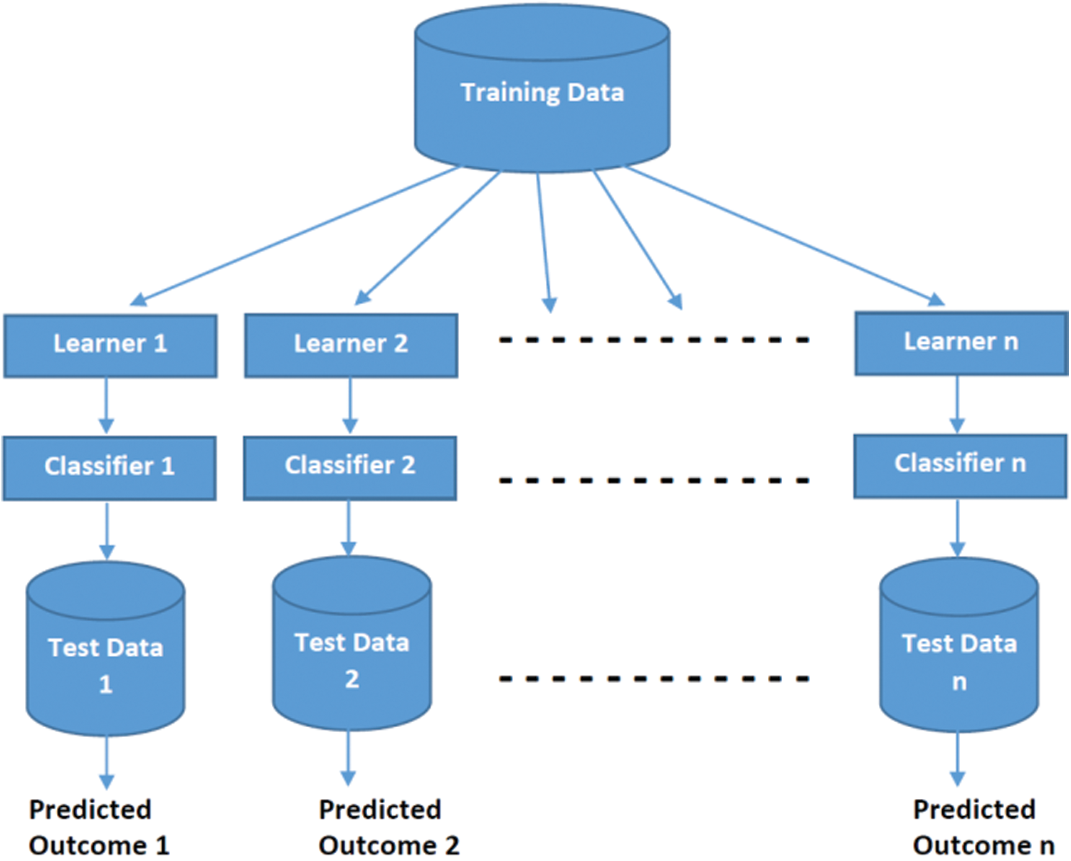
Figure 2: Workflow of base classifiers
6 Base Classification Algorithm
1. Given a set of N points (samples). In this study, we set N = 7.
2. Convert the given set into a training set (70%) and a test set (30%).
3. Apply the same preprocessing on all these datasets.
4. For i = 1 to N do.
5. For j = 1 to M do.
6. Apply Classifier g(i) on Dataset(j)
7. End for
8. Save prediction [i, j]
9. End for
Here g(i) is the i-th classifier and Dataset(j) is the j-th dataset. Prediction [i, j] is the results produced by i-th classifier on j-th dataset where i = 1, 2, 3, …, 7 and j = 1, 2, 3.
In this case, N = 7 as there are seven classifiers and M = 3 for three different datasets.
The computational complexity of this Algorithm is O
After simplification, the above expression is O (MN O (Max
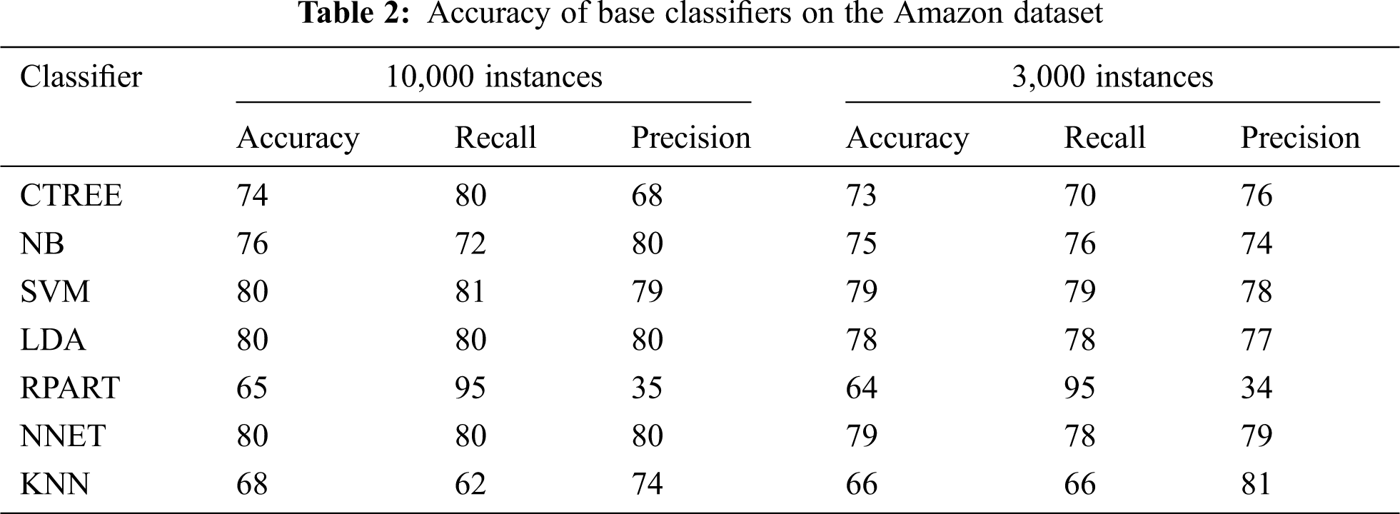
Tab. 1 shows the results of all classifiers on the Amazon Review Dataset with 10000 instances. The three algorithms, i.e., SVM, LDA, and NNET, outperform other algorithms with an accuracy of 80%, whereas NB, CTREE, and KNN get the accuracy of 76%, 74%, and 68% respectively. The RPart performs the worst in this case with an accuracy of 65% only. On the dataset with 3000 instances, it can be seen that SVM and NNET again overtake other classifiers with an accuracy of 79%, whereas LDA, NB, CTREE, and KNN get the accuracy of 78%, 75%, 73%, and 66% respectively. The RPart performs worst again with an accuracy of 64% only.
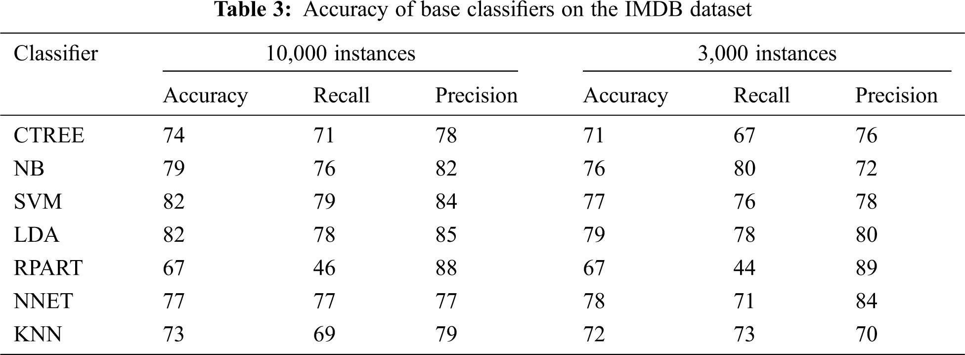
Tab. 2 shows the results of all classifiers on the IMDB Movie Review Dataset with 10000 instances. SVM and LDA outperform other classifiers with an accuracy of 82%, whereas NB, NNET, CTREE, and KNN get the accuracy of 79%, 77%, 74%, and 73% respectively. With 3000 instances, it can be seen that LDA in this case again overtakes other classifiers with an accuracy of 79%, whereas NNET, SVM, NB, KNN, CTREE, and RPart get the accuracy of 78%, 77%, 76%, 72%, 71%, and 67% respectively as shown in Tab. 3.
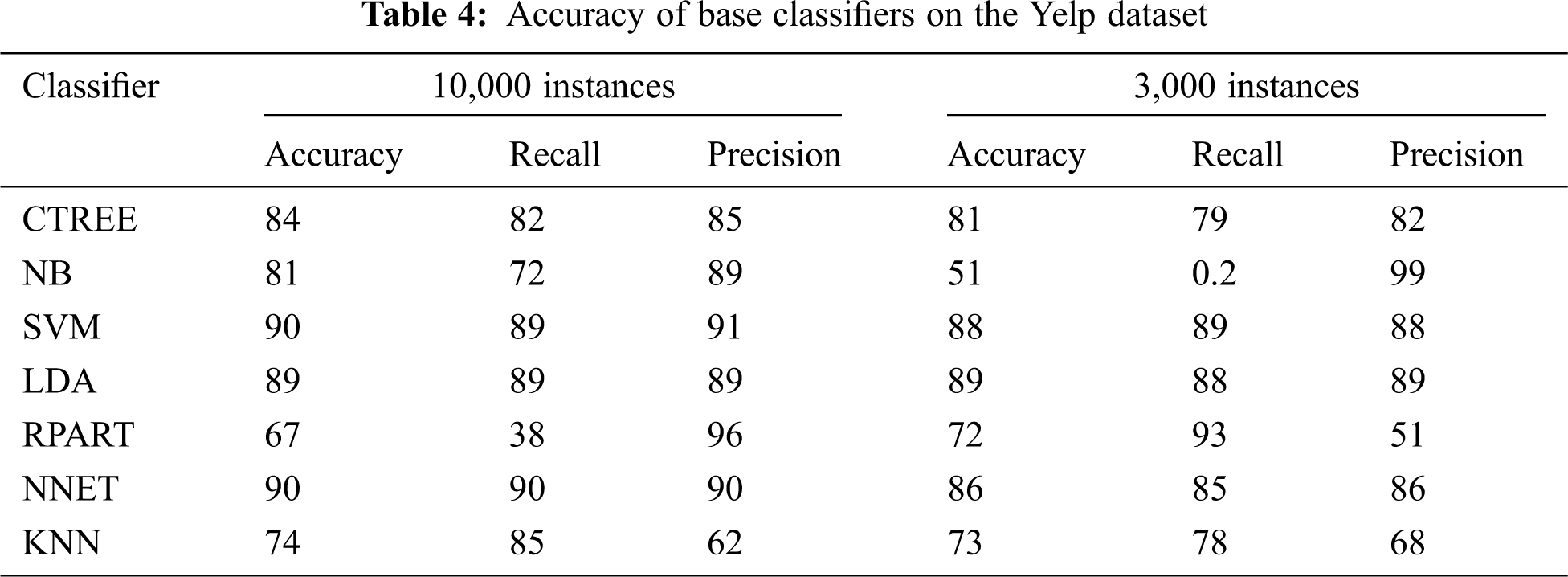
Results of accuracy on different sample sizes of the Yelp dataset also highlight the same issue consistently. It can be seen in Tabs. 4 and 5 that with 10,000 instances, SVM and NNET have better accuracy than other classifiers. LDA performs the best with a 3,000 sample size with an accuracy of 89%. NNET outperforms other classifiers with an accuracy of 87%.
Now if we talk about consistency, it can be observed from the above tables that LDA is more consistent compared to other classifiers.
Another fascinating method in supervised machine learning is to ensemble the predictions of multiple base-level classifiers. The intuition is to acquire a more elevated level of precision at the meta-level than single classifiers. Stacked generalization or stacking is the method that manages the errand of learning meta-level classifiers to join the predictions of various base-level classifiers.
The proposed technique used as shown in Fig. 3, in this study is stacking (also termed as a stacked generalization). The stacking model used in this study is explained below.
In this technique, several classifiers are trained on given data (training set), and their predictions are combined. Metadata is created, and then an algorithm (random or of one’s choice) is trained on this metadata to make a final prediction. In this study, base classifiers LDA, KNN, RPART, SVM, NB, NNET, and CTREE are used at level 1 to predict on three different datasets, i.e., IMDb reviews, Yelp reviews, and Amazon reviews. These predictions are combined to form metadata at level 1 and are used as input at level 2. At this stage, we use all the classifiers at level 1 iteratively to obtain the final prediction. In the stacking process, the input of stage 2 is the output of stage 1 and is learned by some machine learning algorithms at stage 2.
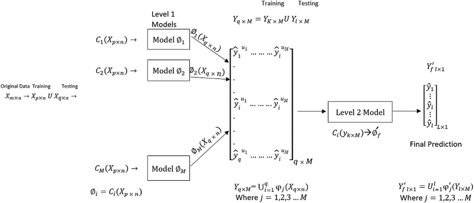
Figure 3: Workflow of the proposed model
In the figure above, X(m×n) represents the original data matrix where m is the number of records (rows) and n is the number of features (columns). Each word of a customer review is taken as a feature in this data after excluding stop words and applying other preprocessing.
Let X(m×n) be a data matrix for classification purposes. The data is divided into training and test sets. Let X(p×n) be the training set, and X(q×n) be the test set for base-level classification, where m = p + q. Here X(m×n) = X U Y, where
The following model illustrates the process of classification at the base level.
where i = 1, 2, …, M.
M denotes the number of classifiers at the base level. Y(q × M) is the output matrix obtained at the base level, consisting of the predictions made by models φi on test data.
Now at the meta-level, data matrix Y(q × M) is used as input. Same base-level classifiers are applied at the meta-level again. So Y(q×M) is again divided into training and test sets. Y(k × M) serves as the training set, and Y(l × M) is used as the test set, where q = l + k.
Following is a figurative illustration of the complete process step by step.
Level 1-Training: As shown in Fig. 4, M different base models ɸ1, ɸ2, …, ɸM are trained using the dataset
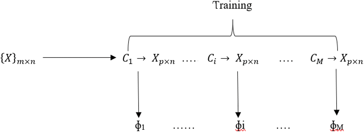
Figure 4: Base level training
Level 1 Test: As shown in Fig. 5, Trained models ɸ1, ɸ2, …, ɸM are applied to test dataset
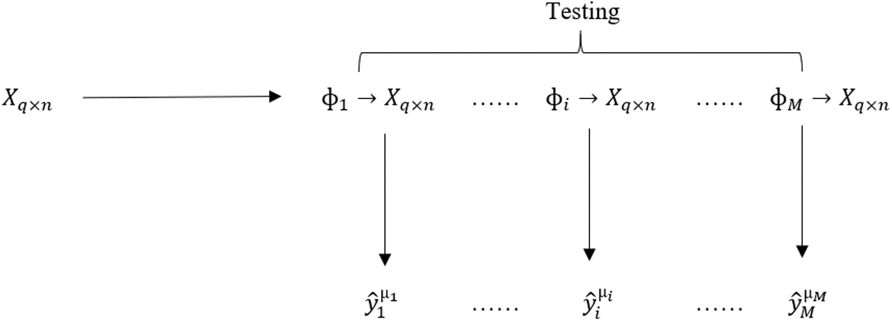
Figure 5: Base level test
Data matrix
Level 2 Training: As shown in Fig. 6, The newly formed dataset
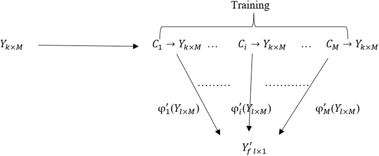
Figure 6: Meta-level training
Mathematically, the whole process can be written as:
Step-1. Ci (
Step-2.
Step-3 Ci (
Step-4
1. //Input training data
2. //Output ensemble classifier H
3. //Step 1: Learn base-level classifiers.
4. for i = 1 to M
5. learn ɸi on
6. end for
7. //Step 2: Construct a new dataset based on the predictions of Step 1
8. XD = { }
9. for i = 1 to m
10. for j = 1 to M
11.
12. End for
13.
14. End for
15. //Step 3: Learn a meta-classifier
16. Learn H =
Return H
The stacking algorithm has a computational complexity of O(NT
9 Comparison of Base Classifiers and Stacked Models


It is clear from the above tables that there is a significant improvement in the accuracy of different datasets. On the Amazon dataset, we can observe 13% improvement when stacked, while the accuracy is 66% only when individually learned with kNN. Also, improvement can be seen after stacking with all other classifiers when compared with individual classifiers. Stacking with SVM and learning with SVM have the same results, i.e., 79%, but stacking with NB and NNET provides 80% accuracy, which is an improvement of 1% as compared with the best individual classifier’s accuracy, i.e., 79% by SVM and NNET.
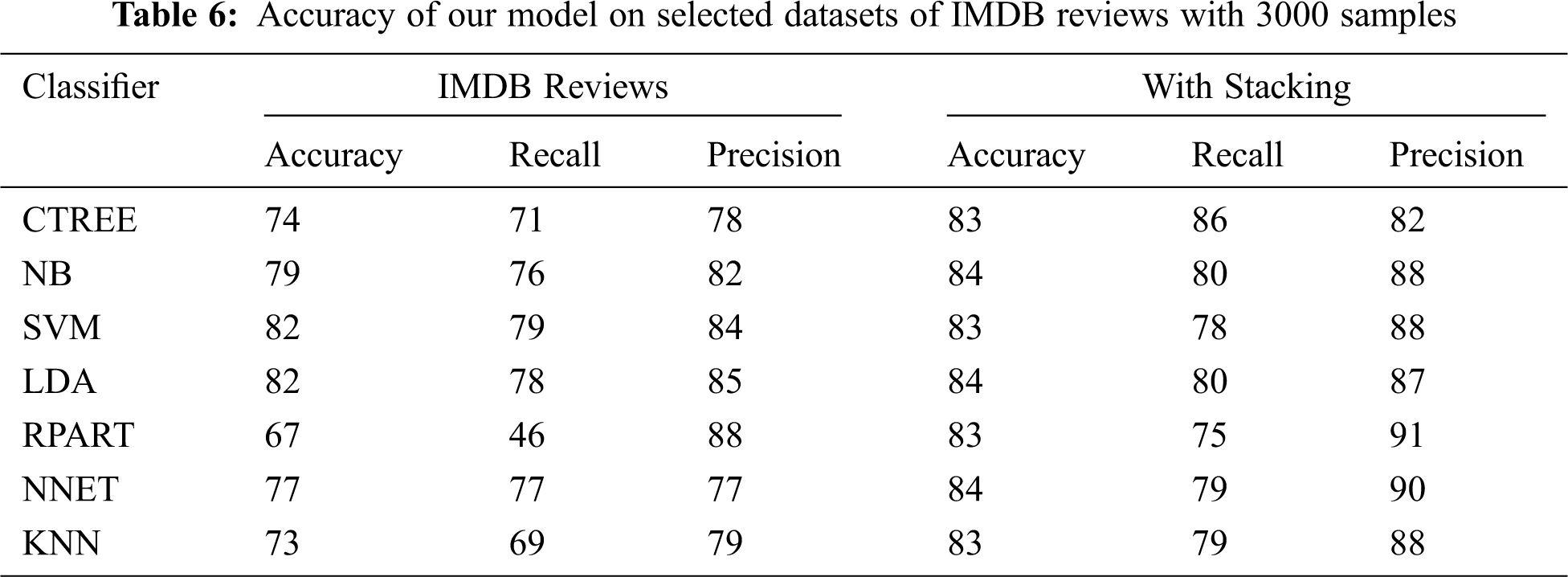
Now take the second dataset IMDB as shown in Tab. 6. It is clear from the above tables that there is quite a significant improvement in accuracy measures. Comparing with individual classifiers, we obtain a slight improvement. The maximum accuracy achieved by individual classifiers is 79%. On the other hand, the best accuracy achieved with stacking is 84%, so a minimum of 5% improvement is achieved on the IMDB dataset. The maximum difference of 16% can be observed when we use the RPART classifier individually and while stacking with RPART. A minimum of 5% improvement can be seen while using LDA individually and while stacking with LDA.
Now let’s consider the third dataset Yelp as shown in Tab. 7. Here the minimum improvement is 1% when LDA is used individually (89%) and after stacking with LDA (90%). And the maximum improvement is 19% while stacking with RPART (91%) and individually (72%). Also, the minimum improvement is 2% considering the overall scenario, i.e., the highest accuracy obtained by individual classifiers is 89% (LDA) and the highest accuracy achieved with stacking is 91% (with RPART).
It is clear from the above comparison tables that better results can be achieved using the stacked generalization. Also, the best accuracy achieved with any sample size can be improved or at least retained when stacked with any of the classifiers at the meta-level. With stacking, both objectives are achieved, i.e., improvement in accuracy and consistency.
Since different sample sizes of three different datasets have been used, we can generalize our conclusion to all binary-class sentiment data.
The main purpose of this research work is to address accuracy improvement and consistency on different sentiment datasets. There are certain models which show excellent results on one dataset but do not perform well on another. So, consistency in accuracy improvement has been a challenge for data scientists. Results obtained from this model are not only better in accuracy but are also more consistent on different instances of different datasets.
A novel heterogeneous ensemble model for the classification of sentiment data is presented in this paper. The investigational results show that the model presented is explicitly viable and effective. It represents its capacity for the vital blend of various classifiers. The model is additionally computationally efficient. However, the computational time complexity matter can be a zone of concern if there is an expanding number of base classifiers in the ensemble along with a huge dataset.
This work has opened many future research venues. For example, one can draw on this research by applying and testing the recommended framework with other sentiment analysis techniques.
Certain areas need to be addressed by researchers. One of them is the relationship between the number of diverse classifiers and accuracy measures. How the number of features is reduced without compromising the quality of tokens can be another zone to be explored, as it can be of great help in optimizing the computational complexity.
Acknowledgement: We appreciate the linguistic assistance provided by TopEdit (www.topeditsci.com) during the preparation of this manuscript.
Funding Statement: The author(s) received no specific funding for this study.
Conflicts of Interest: The authors declare that they have no conflicts of interest to report regarding the present study.
1. A. Gustavsson, L. Jonsson, T. Rapp, E. Reynish, P. J. Ousset et al., “Differences in resource use and costs of dementia care between European countries: Baseline data from the ICTUS study,” Journal of Nutrition, Health and Aging, vol. 14, no. 8, pp. 648–654, 2010. [Google Scholar]
2. L. Piyathilaka and S. Kodagoda, “Human activity recognition for domestic robots,” Springer Tracts in Advanced Robotics, vol. 105, no. 7, pp. 395–408, 2015. [Google Scholar]
3. W. Hussain, M. T. Sadiq, S. Siuly and A. U. Rehman, “Epileptic seizure detection using 1 D-convolutional long short-term memory neural networks,” Applied Acoustics, vol. 177, no. 9, pp. 682–698, 2021. [Google Scholar]
4. A. Mihoub and G. Lefebvre, “Wearables and social signal processing for smarter public presentations,” ACM Transactions on Interactive Intelligent Systems, vol. 9, no. 2–3, pp. 9–32, 2019. [Google Scholar]
5. A. Tripathy and S. K. Rath, “Classification of sentiment of reviews using supervised machine learning techniques,” International Journal of Rough Sets and Data Analysis, vol. 4, no. 1, pp. 56–74, 2017. [Google Scholar]
6. L. Li, T. T. Goh and D. Jin, “How textual quality of online reviews affect classification performance: A case of deep learning sentiment analysis,” Cognitive Computing for Intelligent Application and Service, vol. 32, no. 2, pp. 4387–4415, 2018. [Google Scholar]
7. M. Rathi, A. Malik, D. Varshney, R. Sharma and S. Mendiratta, “Sentiment analysis of tweets using machine learning approach,” in Proc. Eleventh Int. Conf. on Contemporary Computing, Noida, India, pp. 1–3, 2018. [Google Scholar]
8. A. Prabhat and V. Khullar, “Sentiment classification on big data using Naïve Bayes and logistic regression,” in Proc. Int. Conf. on Computer Communication and Informatics, Coimbatore, India, pp. 1–5, 2017. [Google Scholar]
9. M. Bouazizi and T. Ohtsuki, “A pattern-based approach for multi-class sentiment analysis in twitter,” IEEE Access, vol. 5, no. 5, pp. 20617–20639, 2017. [Google Scholar]
10. H. Akbari, M. T. Sadiq, A. U. Rehman, M. Ghazvini, R. A. Naqvi et al., “Depression recognition based on the reconstruction of phase space of EEG signals and geometrical features,” Applied Acoustics, vol. 179, no. 3, pp. 108078–108091, 2021. [Google Scholar]
11. L. Nguyen, “Tutorial on hidden Markov model,” Applied and Computational Mathematics, vol. 6, no. 4, pp. 16–38, 2016. [Google Scholar]
12. F. J. Ordóñez, P. D. Toledo and A. Sanchis, “Activity recognition using hybrid generative/discriminative models on home environments using binary sensors,” Sensors, vol. 13, no. 5, pp. 5460–5477, 2013. [Google Scholar]
13. Z. Fan, M. Jamil, M. T. Sadiq, X. Huang and X. Yu, “Exploiting multiple optimizers with transfer learning techniques for the identification of COVID-19 patients,” Journal of Healthcare Engineering, vol. 9, no. 4, pp. 1–13, 2020. [Google Scholar]
14. C. J. C. Burges, “A tutorial on support vector machines for pattern recognition,” Data Mining and Knowledge Discovery, vol. 2, no. 2, pp. 121–167, 1998. [Google Scholar]
15. H. Akbari, M. T. Sadiq and A. U. Rehman, “Classification of normal and depressed EEG signals based on centered correntropy of rhythms in empirical wavelet transform domain,” Health Information Science and Systems, vol. 9, no. 9, pp. 254–269, 2021. [Google Scholar]
16. U. A. B. U. A. Bakar, H. Ghayvat, S. F. Hasanm and S. C. Mukhopadhyay, “Activity and anomaly detection in smart home: A survey,” Next Generation Sensors and Systems, vol. 16, no. 1, pp. 191–220, 2016. [Google Scholar]
17. C. Debes, A. Merentitis, S. Sukhanov, M. Niessen, N. Frangiadakis et al., “Monitoring activities of daily living in smart homes: Understanding human behavior,” IEEE Signal Processing Magazine, vol. 33, no. 2, pp. 81–94, 2016. [Google Scholar]
18. G. S. Chauhan, Y. K. Meena, D. Gopalani and R. Nahta, “A two-step hybrid unsupervised model with attention mechanism for aspect extraction,” Expert Systems with Applications, vol. 161, no. 1, pp. 1–16, 2020. [Google Scholar]
19. A. U. Rehman, M. T. Sadiq, N. Shabbir and G. Jafri, “Opportunistic cognitive MAC (OC-MAC) protocol for dynamic spectrum access in WLAN environment,” International Journal of Computer Science Issues, vol. 19, no. 3, pp. 395–409, 2013. [Google Scholar]
20. A. Jalal, S. Kamal and C. A. Azurdia-Meza, “Depth maps-based human segmentation and action recognition using full-body plus body-color cues via recognizer engine,” Journal of Electrical Engineering & Technology, vol. 14, no. 1, pp. 455–461, 2019. [Google Scholar]
21. M. T. Sadiq, X. Yu, Z. Yuan, Z. Fan, A. U. Rehman et al., “Motor imagery EEG signals classification based on mode amplitude and frequency components using empirical wavelet transform,” IEEE Access, vol. 14, no. 6, pp. 1–15, 2019. [Google Scholar]
22. H. A. Mengash and A. Hannan, “Methodology for detecting strabismus through video analysis and intelligent mining techniques,” Computers Materials and Continua, vol. 67, no. 1, pp. 1013–1032, 2021. [Google Scholar]
23. M. Valdivia, E. Cámara, J. M. P. Ortega and L. A. Ureña-López, “Sentiment polarity detection in Spanish reviews combining supervised and unsupervised approaches,” Expert Systems with Applications, vol. 40, no. 10, pp. 3934–3942, 2012. [Google Scholar]
24. D. Zhang, H. Xu, Z. Su and Y. Xu, “Chinese comments sentiment classification based on word2vec and SVM,” Expert Systems with Applications, vol. 42, no. 4, pp. 1857–1863, 2015. [Google Scholar]
 | This work is licensed under a Creative Commons Attribution 4.0 International License, which permits unrestricted use, distribution, and reproduction in any medium, provided the original work is properly cited. |