DOI:10.32604/iasc.2021.019727
| Intelligent Automation & Soft Computing DOI:10.32604/iasc.2021.019727 | |
| Article |
Adversarial Examples Generation Algorithm through DCGAN
1School of Computer Science, Southwest Petroleum University, Chengdu, 610500, China
2AECC Sichuan Gas Turbine Establishment, Mianyang, 621700, China
3Department of Computer Science, Brunel University London, Middlesex, UB8 3PH, United Kingdom
*Corresponding Author: Desheng Zheng. Email: zheng_de_sheng@163.com
Received: 23 April 2021; Accepted: 06 July 2021
Abstract: In recent years, due to the popularization of deep learning technology, more and more attention has been paid to the security of deep neural networks. A wide variety of machine learning algorithms can attack neural networks and make its classification and judgement of target samples wrong. However, the previous attack algorithms are based on the calculation of the corresponding model to generate unique adversarial examples, and cannot extract attack features and generate corresponding samples in batches. In this paper, Generative Adversarial Networks (GAN) is used to learn the distribution of adversarial examples generated by FGSM and establish a generation model, thus generating corresponding adversarial examples in batches. The experiment shows that using the Unsupervised Representation Learning with Deep Convolutional Generative Adversarial Networks (DCGAN) to extract and learn the attack characteristics from the FGSM algorithm, the generated adversarial examples attacked the original model with a success rate of 89.1%. For the model attack with increased protection, the success rate increased by 30.3%. This suggests that the adversarial examples generated by GAN are more effective and aggressive. This paper proposes a new approach to generate adversarial examples.
Keywords: Adversarial examples; GAN; deep learning; FGSM algorithm; MNIST dataset
With the development of information technology rapidly, deep learning is gradually being recognized and accepted. In many domains, deep learning can complete preset tasks outerform traditional methods, achieving even human-competitive results. However, while deep learning technology is widely used, the importance of its security cannot be overlooked.
According to research, existing deep neural networks are fragile and vulnerable to attacks. Szegedy et al. [1] first found that in the field of image recognition, only a very slight modification on the image will cause the classifier to misclassify the instances. In fact, these modifications make deep neural networks (DNNs) vulnerable to attacks. As the attack algorithms become more and more advanced, the adversarial example becomes more and more aggressive and produces more and more damage. As shown in Fig. 1:
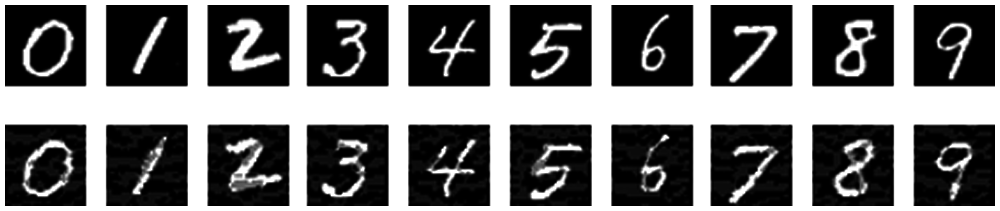
Figure 1: Comparison of adversarial examples and original images
The picture at the bottom is generated by a certain algorithm from the picture at the top, and the neural network will classify it incorrectly. This is very dangerous since deep learning has widely used in security-sensitive fields such as unmanned vehicles, face recognition, bank identity recognition, etc. Therefore, it’s necessary to research on what mentioned above. This research direction is called Adversarial Machine Learning (AML), which means that the target model will misclassify the data under the intentional design of the attacker.
In recent years, a large number of papers about adversarial examples and GAN have been published.
In the aspect of adversarial examples, since 2014, Szegedy et al. [1] proposed the concept of adversarial examples and proposed the L-BFGS algorithm for the first time. He pointed out that deep neural network is highly expressive model but this high expressive force also leads to its counter-intuitive properties: the input-output mapping learned by the deep neural network is discontinuous to a large extent, so the network can misclassify the image by applying some imperceptible perturbations which is found by maximizing the prediction error of the network. Goodfellow et al. [2] proposed FGSM, a fast and efficient attack algorithm, as well as a defense idea, which can be summarized as follows. Let’s say there is an input instance
In the field of GAN, Goodfellow et al. [12] proposed Generative Adversarial Network in 2014. In this paper, he analyzed the advantages and disadvantages of GAN and pointed out the future research direction and expansion. In the same year, Mirza et al. [13] and others proposed a conditional generative adversarial network, which is a conditional version of the GAN. It is proved that CGAN can generate MNIST digits based on class labels. Arjovsky et al. [14] published a paper in 2017, which introduced WGAN. In this paper, he used the theory of maximum likelihood estimation to explain the significance of learning probability distribution in unsupervised learning, used one division to approximate the true distribution, and solved it by minimizing two KL divergence between distributions. Li et al. [15] pointed out that although progress has been made in generating image modeling, it is still an elusive goal to successfully generate high-resolution and diverse samples from complex data sets such as ImageNet [16]. Therefore, they proposed applying orthogonal regularization to the generator to make it suitable for simple “truncation techniques”, allowing precise control of the trade-off between sample fidelity and variation by truncating the latent space. Such modification led to the model reaching a new level of technology in image synthesis under category conditions. Zhang et al. [17] proposed an alternative generator architecture for generative adversarial networks. This new architecture [18] is able to control the high-level attributes of the generated image, such as hairstyle, freckles. The generated image scores better on some evaluation criteria.
The previous adversary algorithms are directly generated by neural networks, while the algorithm proposed in this paper is based on the generated adversarial examples extracting features through GAN networks, which can generate similar adversarial samples in batches with effectiveness and high aggressiveness.
Ian Goodfellow [2] found that the accuracy of a single input function is limited in many problems. For example, they usually use only 8 bits per pixel in digital images domain, so they discard all information below 1/255 of the dynamic range. Owing to the features of limited accuracy, in the case of inputting
Consider the dot product between the weight vector
Adversarial disturbances increase the activation value by
That is to say, if the input of the simple linear model has sufficient dimensions, adversarial examples can be generated. Under this condition, suppose that
Since n-dimensional gradient calculation is applied in the formula, this algorithm is called Fast Gradient Sign Method (FGSM) [19], which can use backpropagation [20] to efficiently calculate the required gradient.
DCGAN is a new method after Ian J. Goodfellow's pioneering GAN in his paper in 2014 that combines GAN and convolutional networks to solve the instability of GAN training [21]. CNN has made great achievements in the field of supervised learning for a long time, such as large-scale image classification and target detection, but has not made particular progress in the field of unsupervised learning [22], which inspired Alec Radford proposed DCGAN, which combines CNN with GAN, and demonstrated its impressive achievements in unsupervised learning [23]. Through training on a large number of different data sets, it is fully demonstrated that the generator and discriminator of DCGAN have learned a rich level of expression in terms of object components and scenes [24].
The main reasons why DCGAN can improve the stability of GAN training are as follows:
1. Use step-size convolution instead of the up-sampling layer [25]. Convolution has a good effect in extracting image features, and convolution is used to instead the fully connected layer.
2. Almost every layer in the generator G and the discriminator D uses the batch normalization layer to normalize the output of the feature layer together, which speeds up the training and improves the stability of the training.
3. The LeakyRelu activation function is used in the discriminator instead of the Relu activation function to prevent gradient sparseness. Relu is still used in the generator, but Tanh is used in the output layer [26].
4. Use Adam optimizer to train, and the best learning rate is 0.0002.
In order to improve the robustness of the neural network, the neural network can be regularized to a certain extent by training a mixture of adversarial examples and legal examples. This form of data augmentation uses inputs that are unlikely to occur naturally, but exposes flaws in the way the model conceptualizes its decision-making function. The FGSM-based countermeasure objective function training is shown in the Eq. (3):
When the data is disturbed by counter disturbances, the counter training process can be seen as trying to minimize the worst-case error. This training process can be interpreted as adding the noise with
In the remaining of the paper we use the following notation:
M* represents the neural network model trained by *, T(*) stands for training on the * data, FGSM(M*) denotes the FGSM attack against the * model, D(*) signifies the adversarial sample generated by *, G(*) symbolizes the DCGAN generator trained by *.
1.
2.
3.
4.
5.
6.
7.
8.
9.
10.
In order to verify the effectiveness and offensiveness of generating new adversarial examples in the DCGAN, the experiment is divided into two parts:
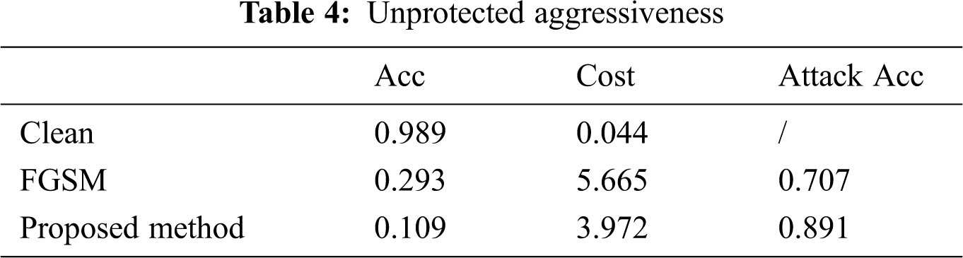
3.2.1 Unprotected Aggressiveness
The initial model
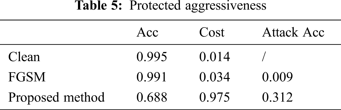
3.2.2 Protected Aggressiveness
The MNIST dataset is trained according to the model set in Section 4.2.2, and the corresponding adversarial training is performed on the model at the same time, and the model
The operating system used in the experiment is Ubuntu 18.04, the CPU is Intel Xeon(R)CPU E5-2609 v4 @ 1.70 GHz, the GPU is Nvidia 1080Ti with 8 GB of memory.
MNIST (Mixed National Institute of Standards and Technology database) is a computer vision data set that contains 70,000 gray-scale pictures of handwritten numbers, each of which contains 28 × 28 pixels. Each picture has a corresponding label. The data set is divided into two parts: a training data set of 60,000 rows and a test data set of 10,000 rows. Among them: the training set of 60000 rows is divided into the training set of 55000 rows and the verification set of 5000 rows. The MNIST data set is widely used in the domain of deep learning and computer vision.
There are three kinds of neural network models in this experiment, which respectively are used for CNN model training, DCGAN generator and DCGAN discriminator construction.
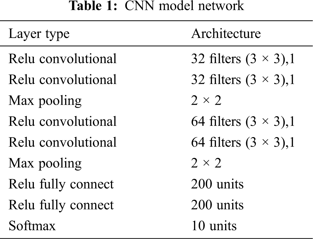
In the CNN model, it is composed of two convolution kernels with 32 filters and a 3 × 3 size, a convolution layer with a step size of 1, two 64 filters immediately after the maximum pooling, and a 3 × 3 convolution kernel, the convolutional layer of the convolutional layer with a step size of 1, two 200-unit full units after the maximum pooling and a 10-unit Softmax fully connected layer for classification, as shown in Tab. 1.
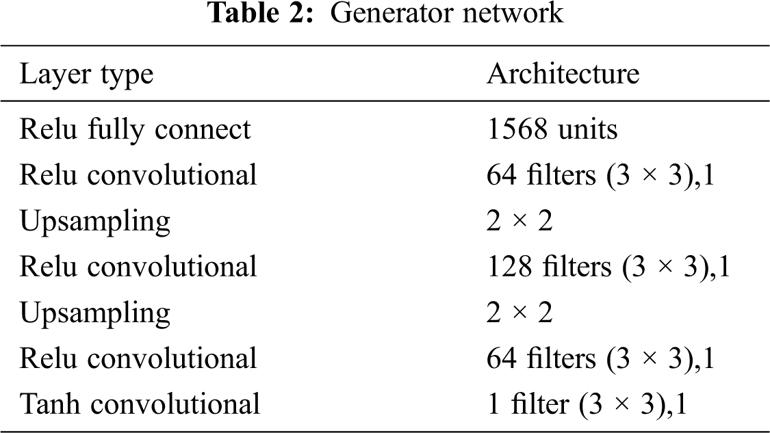
The generator consists of 1568 units fully connected, 64 filters, 3 × 3 size convolution kernel, step size 1 convolution layer, upsampling layer, 128 filters, 3 × 3 size convolution kernel, step size 1 convolution layer, upsampling layer, 64 filters, 3 × 3 size convolution kernel, step size 1 convolution layer, 1 filter, 3 × 3 size convolution kernel, step size 1 convolution layer, as shown in Tab. 2;
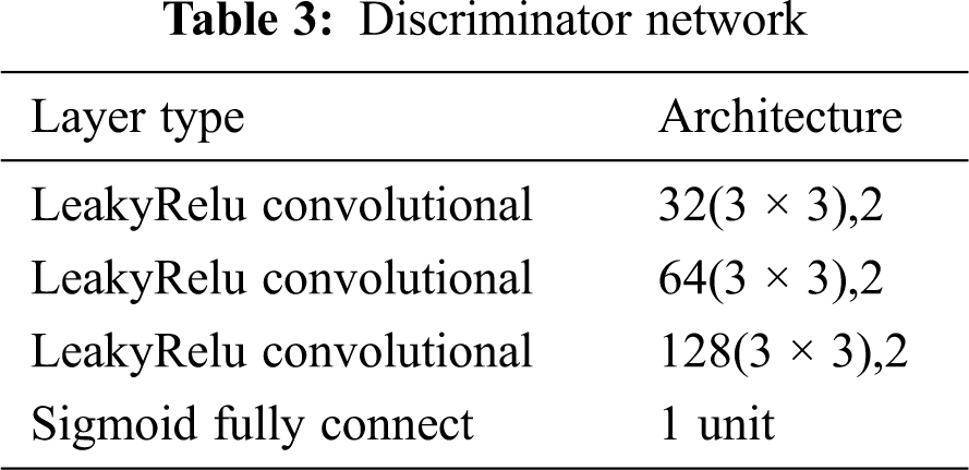
Discriminator is consists of three convolutional layers and a fully connected layer. The three convolutional layers are respectively 32, 64, and 128 filters, a 3 × 3 size convolution kernel, and a step size of 2.
The specific and detailed structural parameters of these three networks are shown in Tabs. 1–3:
The evaluation indicators of this article are as follows:
TP: Positive examples of correctly classified
FN: Positive cases that are misclassified
TN: Negative cases that are correctly classified
FP: Negative cases that are misclassified
The cost function we use is cross entropy function:
Aiming at the effectiveness and aggressiveness of adversarial examples, the experiment was divided into two groups.
Tab. 4 shows the results of the experiment in Fig. 2. The MNIST original images reduce the classification accuracy from 0.99 to 0.29 through the adversarial examples generated by FGSM, and the confidence of adversarial examples generated by DCGAN is 0.11, which shows the effectiveness of the adversarial examples generated by DCGAN.
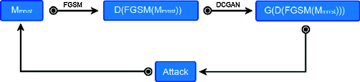
Figure 2:
Tab. 5 corresponds to the results of the experiment in Fig. 3. After the model
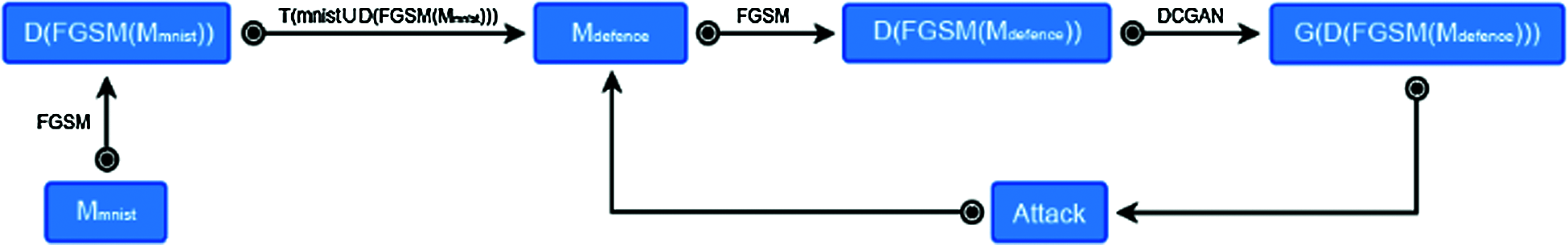
Figure 3:
In this paper, in-depth research on adversarial algorithms is conducted to find a method to generate adversarial examples in batches. Considering the idea of GAN, the application of DCGAN is proposed to learn features of adversarial examples generated by the FGSM algorithm, so that adversarial examples can get rid of the dependence on the original samples and the database, and can automatically generate adversarial examples with the same characteristics. The article introduces the method and effect of the adversarial algorithm attacking the neural network, the protection of the neural network and the method of GAN learning from the adversarial examples in two cases. Experiments show that DCGAN can learn the attack features in adversarial examples and generate adversarial examples in batches. If the model has been trained in the corresponding adversarial, using DCGAN to generate adversarial examples can improve the aggression of the original attack method. In recent years, GAN technology and adversarial learning technology have developed rapidly. There are more than 200 types of networks in the GAN field with diverse performances. With the emergence of attack methods in adversarial learning, there will be more and more options for combining GAN with adversarial learning. Although this article points out the feasibility of combining GAN with adversarial learning, there are still some shortcomings in generality. In the next stage, we will actively seek more options and improve the performance of the attack model.
Funding Statement: This work was supported by Scientific Research Starting Project of SWPU [Zheng, D., No. 0202002131604]; Major Science and Technology Project of Sichuan Province [Zheng, D., No. 8ZDZX0143]; Ministry of Education Collaborative Education Project of China [Zheng, D., No. 952]; Fundamental Research Project [Zheng, D., Nos. 549, 550].
Conflicts of Interest: The authors declare that they have no conflicts of interest to report regarding the present study.
1. C. Szegedy, W. Zaremba, I. Sutskever and J. Bruna, “Intriguing properties of neural networks,” in Proc. of the Int. Conf. on Learning Representations, Banff, Canada, pp. 461–472, 2014. [Google Scholar]
2. I. J. Goodfellow, J. Shlens and C. Szegedy, “Explaining and harnessing adversarial examples,” in Proc. of the Int. Conf. on Learning Representations, San Diego, CA, USA, pp. 1562–1569, 2015. [Google Scholar]
3. A. Kurakin, I. J. Goodfellow and S. Bengio, “Adversarial examples in the physical world,” in Proc. of the Int. Conf. on Learning Representations, Toulon, TLN, FR, pp. 236–248, 2017. [Google Scholar]
4. N. Papernot, P. Mcdaniel and S. Jha, “The limitations of deep learning in adversarial settings,” in IEEE European Sym. on Security & Privacy, Saarbrucken, ScN, DE, pp. 521–527, 2016. [Google Scholar]
5. J. Su, D. V. Vargas and S. Kouichi, “One pixel attack for fooling deep neural networks,” IEEE Transactions on Evolutionary Computation, vol. 23, no. 5, pp. 828–841, 2019. [Google Scholar]
6. N. Papernot, P. Mcdaniel and X. Wu, “Distillation as a defense to adversarial perturbations against deep neural networks,” in IEEE Sym. on Security & Privacy, California, CA, USA, pp. 842–861, 2016. [Google Scholar]
7. N. Carlini and D. Wagner, “Towards evaluating the robustness of neural networks,” Computer Vision and Pattern Recognition, vol. 5, no. 1, pp. 712–731, 2017. [Google Scholar]
8. S. Moosavi-Dezfooli, A. Fawzi and P. Frossard, “DeepFool: A simple and accurate method to fool deep neural networks,” in Computer Vision and Pattern Recognition. (CVPR), Las Vegas, LV, USA, pp. 2574–2582, 2016. [Google Scholar]
9. S. M. Moosavidezfooli, A. Fawzi and O. Fawzi, “Universal adversarial perturbations,” in Computer Vision and Pattern Recognition. (CVPR), Honolulu, HI, USA, pp. 586–605, 2017. [Google Scholar]
10. S. Sarkar, A. Bansal and U. Mahbub, “UPSET and ANGRI: Breaking high performance image classifiers,” in Computer Vision and Pattern Recognition. (CVPR), Honolulu, HI, USA, pp. 596–622, 2017. [Google Scholar]
11. S. Baluja and I. Fischer, “Learning to generate adversarial examples,” IEEE Transactions on Evolutionary Computation, vol. 23, no. 5, pp. 828–841, 2017. [Google Scholar]
12. I. J. Goodfellow, J. Pougetabadie and M. Mirza, “Generative adversarial networks,” Advances in Neural Information Processing Systems, vol. 5, no. 1, pp. 2672–2680, 2014. [Google Scholar]
13. M. Mirza and S. Osindero, “Conditional generative adversarial nets,” in Computer Vision and Pattern Recognition. (CVPR), Las Vegas, LV, USA, pp. 2574–2582, 2014. [Google Scholar]
14. M. Arjovsky, S. Chintala and L. Bottou, “Wasserstein GAN,” in Computer Vision and Pattern Recognition. (CVPR), Honolulu, HI, USA, pp. 596–622, 2017. [Google Scholar]
15. X. Li, Q. Zhu and Y. Huang, “Research on the freezing phenomenon of quantum correlation by machine learning,” Computers, Materials and Continua, vol. 65, no. 3, pp. 2143–2151, 2020. [Google Scholar]
16. X. Qu, S. Chen and X. Wang, “A secure controlled quantum image steganography algorithm,” Quantum Information Processing, vol. 19, no. 10, pp. 1–25, 2020. [Google Scholar]
17. J. Zhang and J. Wang, “A survey on adversarial example,” Journal of Information Hiding and Privacy Protection, vol. 2, no. 1, pp. 47–57, 2020. [Google Scholar]
18. A. Razavi and V. D. Oord, “Generating diverse high-fidelity images with VQ-VAE-2,” Advances in Neural Information Processing Systems, vol. 32, no. 5, pp. 1466–1476, 2019. [Google Scholar]
19. Z. Ran, D. Zheng, Y. Lai and L. Tian, “Applying stack bidirectional LSTM model to intrusion detection,” Computers, Materials and Continua, vol. 65, no. 1, pp. 309–320, 2020. [Google Scholar]
20. T. Karras, S. Laine and T. Aila, “A style-based generator architecture for generative adversarial networks,” in Computer Vision and Pattern Recognition. (CVPR), Los Angeles, LA, USA, pp. 4401–4410, 2019. [Google Scholar]
21. X. Y. Li, Q. S. Zhu, C. You and D. S. Zheng, “Researching the link between the geometric and Renyi discord for special canonical initial states based on neural network method,” Computers, Materials and Continua, vol. 60, no. 3, pp. 1087–1095, 2019. [Google Scholar]
22. T. Lu, Z. S. Li and C. L. Xu, “FGSM: A framework for grid service mining,” Journal of Sichuan University, vol. 3, no. 1, pp. 121–129, 2005. [Google Scholar]
23. N. V. Irukulapati, H. Wymeersch and P. Johannisson, “Stochastic digital backpropagation,” IEEE Transactions on Communications, vol. 3, no. 1, pp. 2574–2582, 2002. [Google Scholar]
24. A. Radford, L. Metz and S. Chintala, “Unsupervised representation learning with deep convolutional generative adversarial networks,” Computer Science, vol. 1, no. 4, pp. 89–96, 2015. [Google Scholar]
25. L. S. Meng, K. Ren, C. Q. Fan and L. Huang, “Dense convolution generative adversarial networks based image inpainting,” Computer Science, vol. 47, no. 8, pp. 202–207, 2020. [Google Scholar]
26. P. L. He, Y. X. Shi and J. Cheng, “Face image translation based on generative adversarial text,” Computing Technology and Automation, vol. 37, no. 4, pp. 77–82, 2019. [Google Scholar]
 | This work is licensed under a Creative Commons Attribution 4.0 International License, which permits unrestricted use, distribution, and reproduction in any medium, provided the original work is properly cited. |