DOI:10.32604/iasc.2022.017706
| Intelligent Automation & Soft Computing DOI:10.32604/iasc.2022.017706 | |
| Article |
Plant Disease Classification Using Deep Bilinear CNN
1VNR VJIET, Hyderabad, 500090, India
2Geetanjali College of Engineering and Technology, Hyderabad, 501301, India
3Gokaraju Rangaraju Institute of Engineering and Technology, Hyderabad, 500090, India
4Kakatiya Institute of Technology and Science, Warangal, 506015, India
*Corresponding Author: N. Rajasekhar. Email: rajasekhar531@gmail.com
Received: 08 February 2021; Accepted: 24 April 2021
Abstract: Plant diseases have become a major threat in farming and provision of food. Various plant diseases have affected the natural growth of the plants and the infected plants are the leading factors for loss of crop production. The manual detection and identification of the plant diseases require a careful and observative examination through expertise. To overcome manual testing procedures an automated identification and detection can be implied which provides faster, scalable and precisive solutions. In this research, the contributions of our work are threefold. Firstly, a bi-linear convolution neural network (Bi-CNNs) for plant leaf disease identification and classification is proposed. Secondly, we fine-tune VGG and pruned ResNets and utilize them as feature extractors and connect them to fully connected dense networks. The hyperparameters are tuned to reach faster convergence and obtain better generalization during stochastic optimization of Bi-CNN(s). Finally, the proposed model is designed to leverage scalability by implying the Bi-CNN model into a real-world application and release it as an open-source. The model is designed on variant testing criteria ranging from 10% to 50%. These models are evaluated on gold-standard classification measures. To study the performance, testing samples were expanded by 5x (i.e., from 10% to 50%) and it is found that the deviation in the accuracy was quite low (0.27%) which resembles the consistent generalization ability. Finally, the larger model obtained an accuracy score of 94.98% for 38 distinct classes.
Keywords: Bilinear convolution neural networks (Bi-CNN’s); plant disease classification; mobile API; deep learning; neural networks
Agriculture is the only way for crop production and livelihood. One of the major risk factors of crop productions is dealing with plant diseases. Every single crop produced is linked with a plant disease, which is an obstacle for healthy crop production and this tops the list of reasons for the loss of crop production. If a crop has a plant disease then the symptoms can be noticed by keen observation of different parts of the leaves. Plant diseases are categorized into pests, weeds and plant pathogens. The annually estimated average loss due to pathogens and pests are nearly 13%–22% on the world’s major crop productions like Rice, Wheat, Maize, Potatoes etc. Over the past few decades, farmers used to identify these diseases by observing the leaves through naked-eye. However, this requires the farmer to be extremely skilled or would require the guidance of an agricultural scientist to notice the disease and this process consumes a lot of time.
One of the major reasons for the loss in production is due to diseases like bacterial spot, early blight, late blight, and leaf mould that occur frequently on the leaves of the tomato plant at different stages of its growth. Potatoes are one of the most dominant food crops where the yield of potatoes is reduced by diseases Phytophthora infestans (late blight) and Alternaria solani (early blight). The average yield loss at a global level due to pathogens and pesticides is around 17.2% in potatoes. Apple is been one of the most produced fruits because of its nutritional and medicinal importance where the severity caused by the diseases (Mosaic, Rust, Brown spot, and Alternaria leaf spot) on apple leaves led to huge production and economic loss which also affected the quality in production. Early detection of these types of conditions in the plants that are unhealthy allows us to take precautionary measures and alleviate the production of crops.
In this research, we mainly focus on developing automatic, accurate and less expensive Restful-API into a Mobile-App to detect and classify variant kinds of leaves using Bi-Linear Convolution Neural Networks (Bi-CNNs). The contributions to the body of the knowledge are mentioned as,
1. We propose a bi-linear convolution neural network (Bi-CNNs) for plant disease identification and classification with a leaf images as input.
2. Secondly, we fine-tune VGG and pruned ResNets and utilize them as feature extractors and they’re connected to fully connected dense networks. The hyperparameters are tuned to reach faster convergence and obtain better generalization during stochastic optimization of Bi-CNN(s).
3. Lastly, the proposed model is designed to leverage scalability by implying the Bi-CNN model into a real-world application and release it as an open-source. The detailed explanations of the product are mentioned in the last section.
The design paradigm of the proposed architecture is motivated by the two distinct cortical pathways of the human brain. These two cortical pathways oblige to understand the object vision and spatial vision separately. The occipitoparietal, the dorsal system, helps understand the visual location of the targeted object whereas, the occipitoparietal, the ventral stream, extracts the visual representations of objects i.e., identifying the objects [1]. These two critical pathways extract the information regarding an object from retrieval input to the striate cortex at a juncture. But, the occipitotemporal pathway interconnects the striate the pre-striate and activated to inferior temporal regions which eventually helps to identify the visual stimulus understanding the physical properties of the targeted object.
Further, the occipital parietal pathway the striate then pre-striate are activated to inferior parietal areas which help to localize the visual stimulus i.e., understanding the spatial location of the targeted object. Finally, the two cortical pathways are reintegrated by providing selective attention by adjoining the visual stimulus. These 2 selective attentions are provided to the external feature representation such as color, shape and spatial locations. These activations are seen in the exhaustive cortex. Thus, the neural architecture provides selective attention from the learned representations [2].
The main motive of this research is to provide an application-oriented deep bi-linear convolution neural network that provides selective attention in the neural network by adapting a neuroscience perspective for classifying distinct plant leaves from their infection classes. The mathematical study is furnished in the methodology section.
Siddharth et al. [3] developed a model for the identification and classification of diseases in plant leaf images. The proposed model is based on Radial Basis Function Neural Network (BRBFNN) which uses bacterial foraging for optimization and increases the training speed of the network. The algorithm (Bacterial Forging) searches for the common attribute by the grouping of seed points for identifying the features. Their classification results are based on validation evaluation partition coefficient (Vpc) and validation evaluation partition entropy (Vpe). They also compared their model with traditional machine learning methods such as K-means and SVM. The specificity of the proposed model for segmentation is 0.558 and for classification upon Vpc and Vpe is 0.8621 and 0.1118 respectively.
Aydin et al. [4] has experimented on various transfer learning models to analyze the classification performance. During experimentation, they have four models and analyzed this performance on publicly available datasets. Additionally, they have proposed a CNN model adjoined with LDA to classify the deep featured extracted from the pre-trained network (AlexNet & VGG16). To analyze the performance of the model five-fold cross-validation procedure was adapted and the input size of an image was considered as 100 × 100. The proposed model obtained an accuracy score of 96.93% whereas the pre-trained VGG16 model outperformed with an accuracy of 99.80%. Karthik et al. [5] has researched tomato leaves diseases and proposed two variant CNN architectures. with the help of Residual Progressive Feature Extraction, the model has extracted spatial features with 0.6M parameters. By performing five-fold cross-validation the model obtained an accuracy of 98%.
Mohanty et al. [6] performed experimentation on plant village dataset by using AlexNet & GoogleNet.By contemplating variant types GoogleNet got an accuracy of 98% on grayscale, 99.34% on colour, and 99.25% on segmented images with 5 different splits on 20% test samples. Uday Pratap et al. [7] Multilayer Convolutional Neural Network (MCNN) for classification of mango leaves that are infected with anthracnose disease. The dataset consists of 1070 images of mango leaves which is a real-time dataset captured in a university. The proposed model was validated by 20% test samples and compared with various machine learning techniques. The MCNN model got an accuracy of 97.13%. Sandeep Kumar et al. [8] has implied a new optimization technique called Exponential Spider Monkey Optimization (ESMO) for plant disease identification. SPAM is applied for feature extraction to classify if a leaf is healthy or diseased. Distinct machine learning models are used to evaluate the performance, it was concluded that SVM outperformed other models with an accuracy of 92.1%.
Qiao Kang et al. [9] proposed a network that uses ResNet50 architectures as a backbone model to diagnose plant disease and severity estimation. The proposed network consists of shuffle units as an auxiliary structure which increases the performance of the model. The dataset was collected from the AI challenger Global AI contest which consists of 7 different plant species with an Image size of 256 × 256 × 3. The proposed method got a classification accuracy of 98% and a recognition accuracy of 99%.
Ahmed et al. [10] introduced a model called CaffeNet, It was built on a Caffe framework to label paddy pest and paddy diseases. This work used a database that has 9 paddy pests and 4 paddy disease classes. The aforementioned model was fine-tuned over 30,000 iterations and obtained an accuracy score of 87%. Islam et al. [11] utilized machine learning algorithm and image preprocessing techniques to segment and identify potato disease from the plant village database. It was observed that SVM had an accuracy of 95% (over 300 images).
The complete data was collected from the open repository [12]. The dataset was publicly available for research and hence can be implied for classification and identification of distinct plant disease which can be achieved by designing a user-friendly mobile application. The experimentation is carried out in three folds. The First experimentation, which is named D1, was carried out in 18 classes. In which there are 9 variant fruit leaf images with healthy and unhealthy kinds. As a note, all the variants of unhealthy classes constructed in D1 contains various types such as early blight, black rot, bacterial spot etc. This means all the infected kinds of plant leaves are considered as an unhealthy class of that particular leaf kind.
Next, the experimentation was carried out (D2) where three variant plant leaf images are considered with their multiple infected classes. Lastly, the experimentation was carried out with (D3) which contains the complete 38 classes. The description of the train and test for D1, D2, and D3 is clearly illustrated below (refer to Tab. 1). The complete partitions of the dataset into D1, D2, and D3 are mentioned in the repository1.

VGG Models were utilized while developing a Bi-CNN model where, the two models considered for extracting features are VGG16 and VGG19. The VGG16 and VGG19 contain consecutive convolution and pooling layers with a depth of 16 and 19 layers respectively. These models are pre-trained on the finest weights. The VGG16 and VGG19 models consume 138.3 and 143.6 Million parameters with an input shape of 224 × 224 with three coloring channels. While developing the Bi-CNN model it is assumed that one of the VGG models do capture spatial invariances and the other captures the location of an entity residing in the image [13].
ResNet Models ResNet models are also considered for feature extraction. Two flavors of ResNet’s are implied which are 50 layers deep and the other is 101 layers deep. These ResNet models can capture the invariances of the input by overcoming the problem of degradation. The deep residual connections help to rectify the vanishing gradients and regulate learning for deeper layers. These ResNets are not only computationally cheap but are much deeper and capable of capturing invariances with greater performance. Hence, the two flavors are implied by pruning the network appropriately [14].
The bottom layers with greater feature maps i.e., 2048 activations are excluded. The ResNet model is pruned by truncating the last four activations. During experimentation, it is observed that these activations (final activations) led to high computations. But the original model performance was higher than that of the pruned model. Hence, the ResNet model was pruned by truncating the last four layers with 512 as final activation maps (similar to that of VGG). Similarly, while developing the Bi-CNN model it is assumed that one of the ResNet models do capture spatial invariances and the other captures the location of an entity residing in the image.
Finally, these models (VGG and ResNet models) are fine-tuned with regulated training procedure to reach faster convergence with greater generalization.
4.3 Bi-Linear Convolution Neural Network (Bi-CNN’s)
As mentioned, Bi-CNN’s are motivated by the visual perception of the human brain through two cortical visual pathways. This motivation led to the design of a neural network that extracts spatial locations of the entity residing in an image and captures the structural invariances. So, to extract features bottleneck activations of the pre-trained network are utilized. A set of features for extracting spatial location and morphology of input are chosen as Net − X and Net – Y [15].
Whereas, in our methodology, we utilize not only pre-trained VGG models (as [15]) but also ResNet’s intermediate activations by cautious architecture pruning. To classify D1 only VGG models i.e., VGG16 and VGG19 are utilized. In the case of D2, Pruned ResNet and also VGG models are utilized. But for D3, only pruned ResNet is employed.
Which can be simplifies as,
where
For a clear understanding, the bottleneck activations extracted from the feature extracting models i.e., fvx and fvy are pooled by implying second-order pooling i.e., outer-product is applied to pool those features to linearize to form fvz as a feature vector. This feature vector contains the fine-grained features and the outer-product is appropriately described below. Next, to regularize the model normalization is adapted. This normalization is processed in three steps i.e., three normalization layers are sequentially attached. The first normalization layer is chosen as either natural logarithm of the square root of the individual features extracted from fvz. So, after the first normalization, the features are followed up with a signed square-root as a normalization step. The mathematical formulation for the signed square-root is described below. Thirdly, the feature vectors are regularized through an l2-normalization constraint. When the non-linearities are not regulated properly the maximum probability mass function for each sample is assigned as logit i.e., activated via sigmoid. These assignments certainly cause fragile activations with a high chance for saddle points.
This scenario can be prevented by choosing l2-normalization as the final activation layer. Hence, these three normalization layers can produce effective outcomes by transforming features into a regulated latent space.
Both the normalizations i.e., square-root and logarithm are chosen. As a note, both the normalizations are not chosen at a time.
where,
Next, these latent representations which capture the information regarding the whole image are to be classified appropriately. Tsung Yu et al. [15] implied SVD and LYAP methods for computing the matrices. They are not end-to-end trained neural architectures. They do not have GPU computation end-to-end where; they only compute the extracted feature vectors by classifying them through CPU. For efficient end-to-end training, a fully connected neural network is chosen with successive dropout and batch normalization layers. The major differences from Tsung Ye et al. [15] is, they implied only VGG as pre-trained network and did not imply end-to-end training via backpropagation. But, in this research, a better feature extractor i.e., ResNet’s are implied with end-to-end training.
As a note, the feature-extraction method is the same for all the models mentioned in Tab. 1. But the final layer activations are varied from 3 to 38 depending upon the model. In the given Fig. 1, it can be observed that N is mentioned at final softmax activation which is chosen based on the specific model to be fine-tuned. The feature extraction part is fine-tuned and the classification part is fully trained. In this complete procedure, the gradient flow in the network is appropriately analyzed.
This section gives a complete illustration of the hyperparameter tuning and optimization of model during the course of training Bi-CNNs. The classification architecture is built by fully connected networks with 256-128-N as the pattern. Where N is number of classes for discriminating the input. Firstly, the feed is activated via ReLU as non-linearity. Further, the batch normalization layer is implied to reduce the problem of covariate shift [16]. Next, a dropout layer is added as a regularization method which eventually reduces overfitting [17]. The drop ratio of neurons for reducing overfitting using dropout is chosen as 30% (which is chosen while optimization). The weights for the initialization of the learning procedure are chosen to be glorot-normal [18].
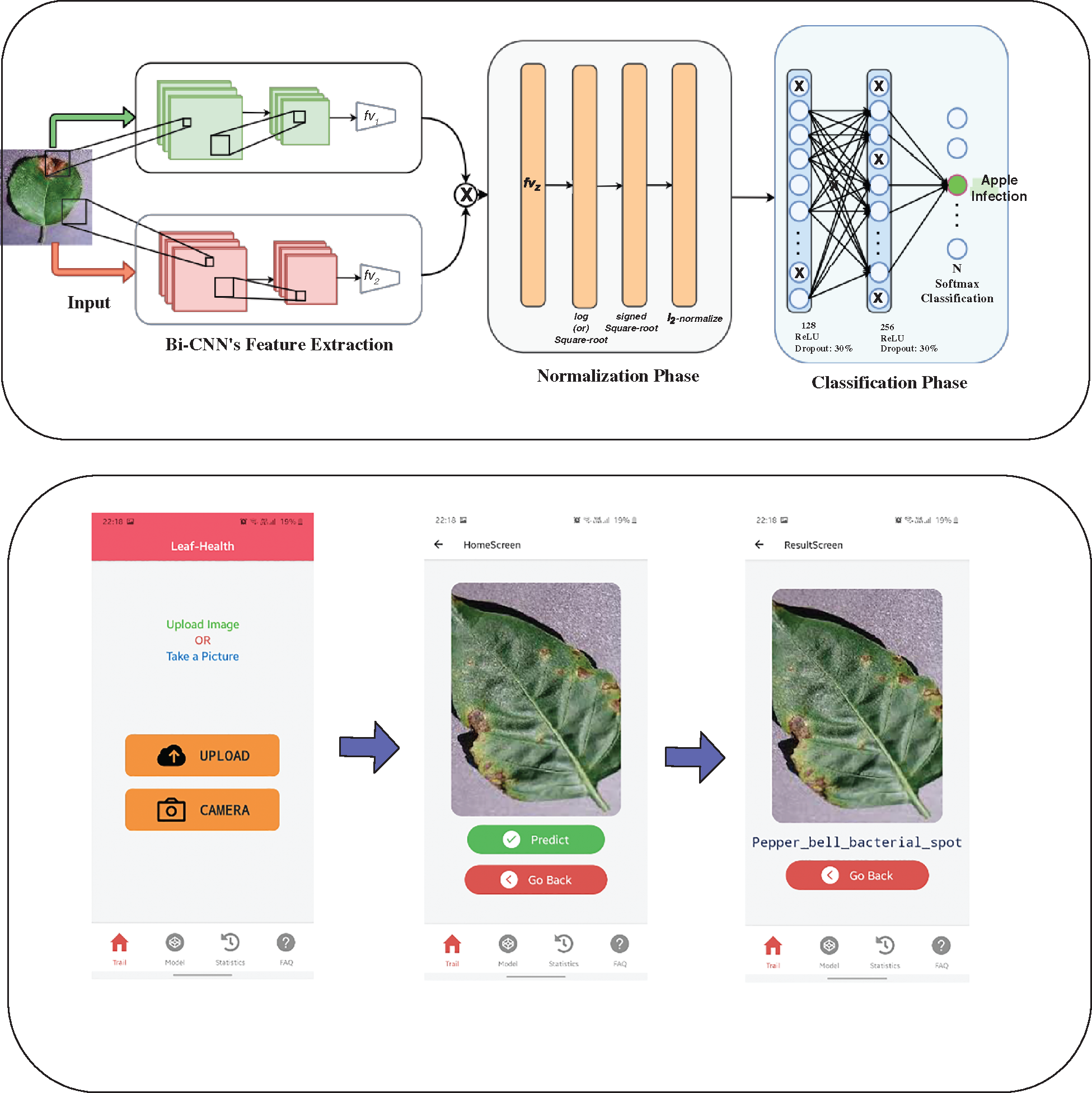
Figure 1: The proposed Bi-linear convolution neural network-integrated in a Mobile App
There are variant models trained. The D1 models are trained using negative log-likelihood as cost function (Loss1). Whereas, for both of the D2, andD3 squared hinge (Loss2) is used as a cost function for stochastic optimization of neural network. The equations are formulated as mentioned as,
where i is no. of instances (feature samples) and k is no. of class labels. y(i) is the ground truth class labels for the class k with an ith instance. y^k(i) is the predicted class label. Further to optimize the model adam [19] is chosen as an optimizer with an initial learning rate of 0.0005. The training schedules are designed by motivating from the work by Samuel L et al. [20]. Where the noise during the training procedure is either reduced by increasing batch size or decaying learning rate (keeping the momentum variable to be constant). The noise during the training is mathematically understood as,
The aim is to decrease noise during training either tweaking the learning rate schedules or batch size. So, slowly increase the learning rate by increasing batch size to obtain faster convergence with greater generalization ability. As the training samples are large regularization provided by l2 would be useful and accordingly learning rates are scheduled [21]. To provide appropriate learning with faster convergence and proper generalization a definite training schedule is obtained, where for every single iteration (≈ 4 epochs) batch size and learning rate are updated cautiously.
At the first iteration, the batch size is initialized as 10 (batch0 ← 10) and the learning rate is initialized as 0.5 × 10⁻³ (rate0 ← 0.5 × 10⁻³). Next, in the second iteration learning is increased to 0.001 and batch size is increased twice of the previous batch i.e., 20. Finally in the third iteration learning is held constant to 0.001 and the batch is increased by 5 units per batch i.e., 25. This iterative computation for stochastic optimization of a neural network is chosen for D1, D2, and D3 respectively. This eventually aided to reach faster convergence with cautious hyperparameter tuning as mentioned2 [22].
To determine the performance of the Bi-CNN’s, classification metrics are implied based on their significance. The metrics such as accuracy score, Receiver operating characteristics (ROC) area under the curve (AUC) [23] and mean-squared error (MSE) are utilized to determine the performance. Accuracy is chosen as the gold standard metric to evaluate classification performance as it aggregates the instances which are correctly classified and divide them with complete instances which are both classified as correct and incorrect.
Next, MSE is utilized as a metric to determine the performance of regression models which observes the deviation from the ground truth to that of predicted instances. So, the deviation can also help determine the performance of the model even when ground truth labels are provided. Finally, AUC is calculated by plotting the true positive rate on the y-axis and the false positive rate on the x-axis. The performance evaluation is carried out by developing variant models as per Tab. 1. The complete result section is divided into two different sections and is are explained below.
In D1 one of the models is produced either by applying square-root as the first normalization layer and the other as a logarithm. Each of the models mentioned in Tab. 1 is evaluated with various metrics. During the evaluation, it is observed that the Bi-CNN model with square-root as the first normalization layer outperformed the logarithm in all of the generalization’s splits.
But, to know whether the proposed model is providing visual attention to the required regions or not heat maps are generated. These heat maps are also known as class activation maps (CAM’s). Heat maps visually describe the final layer activations of the model and impart color to the highly activated regions (i.e., coloring the region of interest). So, to understand these activations from the bottleneck layer fvz heat map is plotted for three different plant leaf kinds (apple, corn, peach) with infection classes and visually depicted in Figs. 2 and 3.
They have the unique property of being insensitive to alterations in the class distributions and can provide good relative instance scores. For handling multiple classes, ROC is calculated by considering one class (chosen) as positive and the remaining classes are considered to be negative ones. So, 18 different AUC-ROC curves are generated. These AUC-ROC curves are generated for the model Bi-CNN (sqrt), as its performance was optimal, for all the generalization splits and visualized in Fig. 4. Further, AUC-ROC curves [23] are generated for an individual class. AUC is used as a metric in Tab. 2 as they provide detailed characteristics of the classifier.
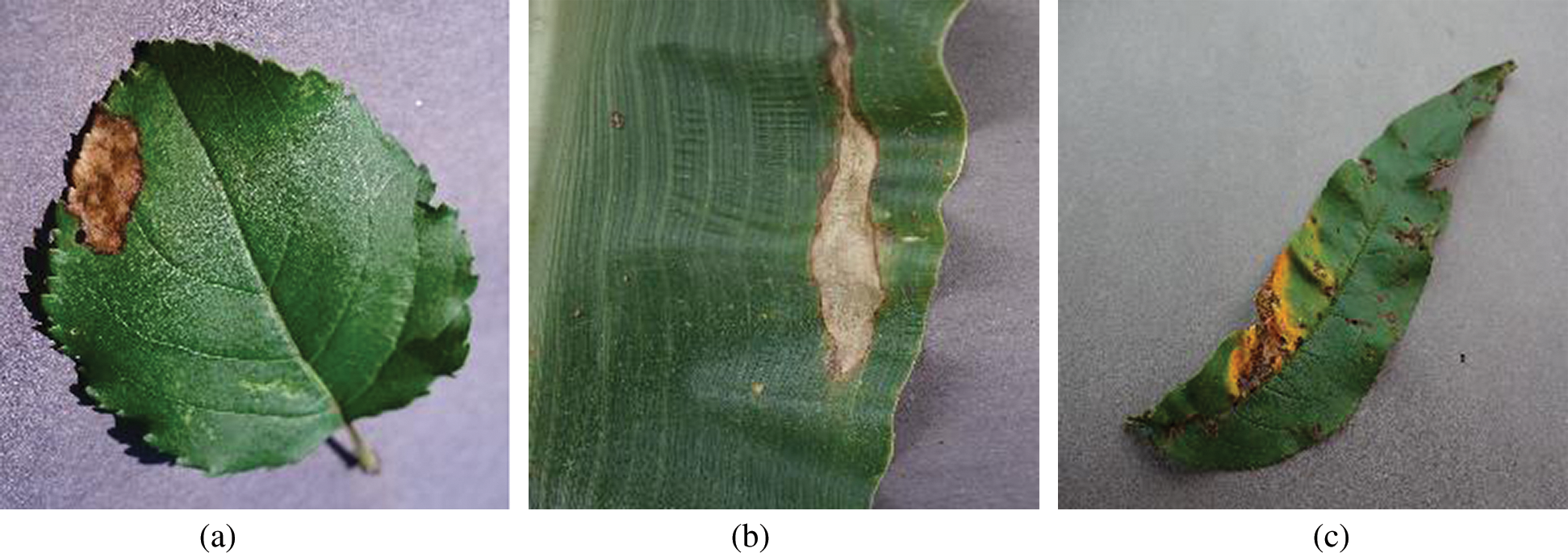
Figure 2: Infected leaves. (a) Unhealthy apple leaf (b) Unhealthy corn leaf (c) Unhealthy peach leaf
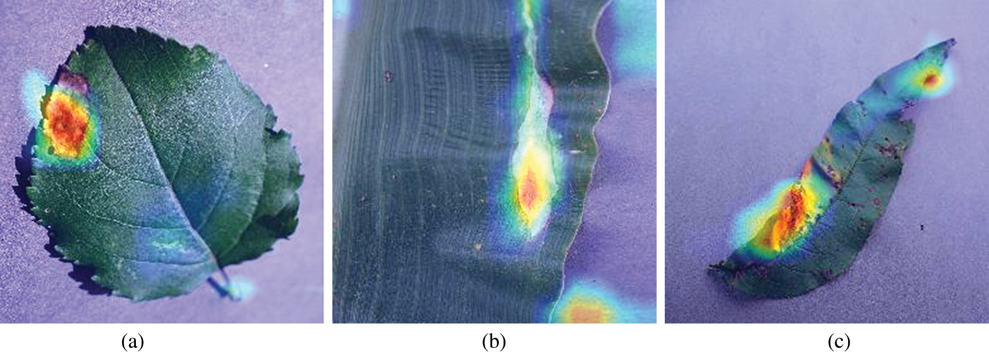
Figure 3: Class activation maps (CAM’s) of Infected leaves. (a) CAM’s of apple infected leaf (b) CAM’s of corn infected leaf (c) CAM’s of peach infected leaf

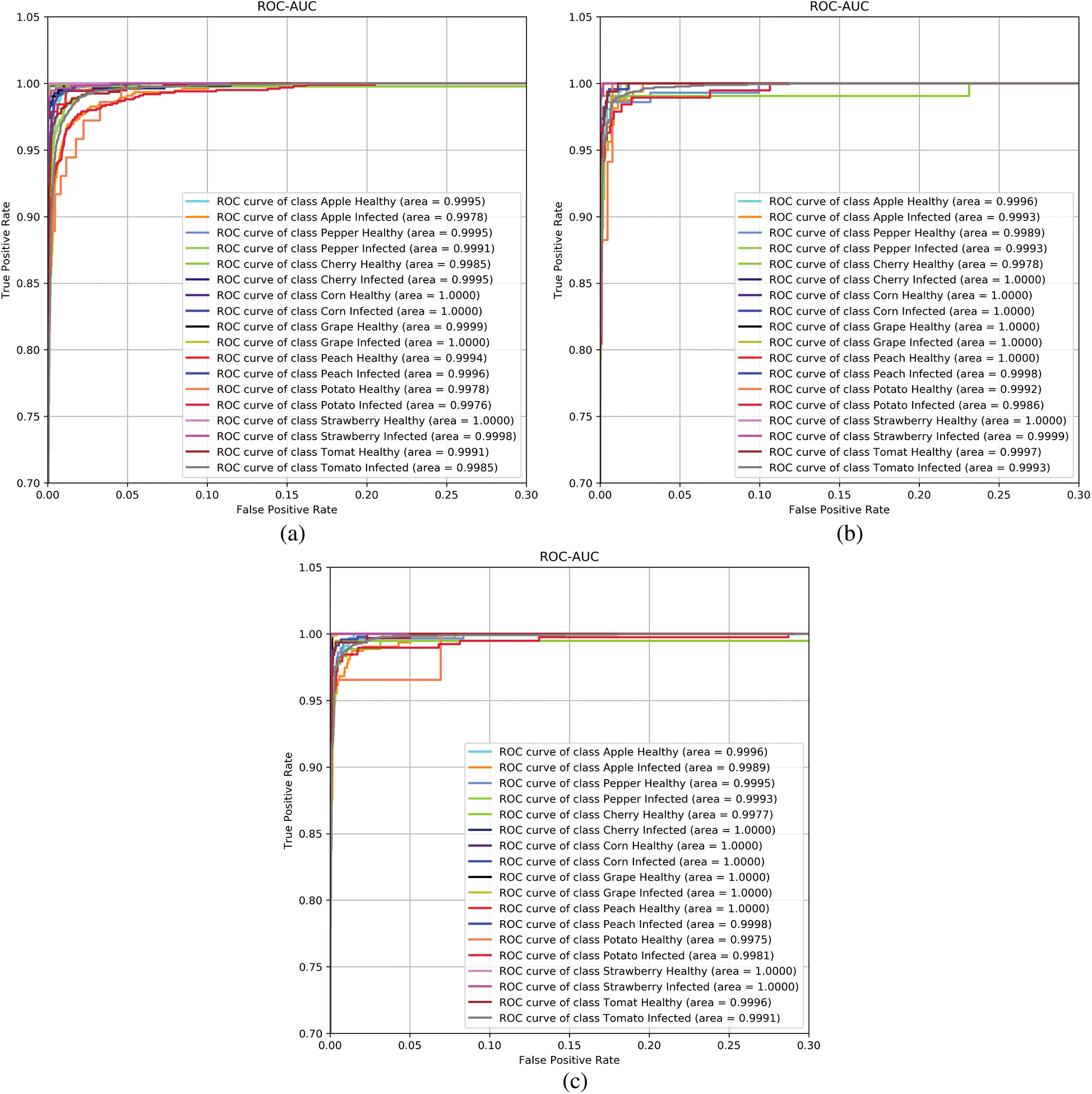
Figure 4: AUC-ROC curves of Bi-CNN’s(sqrt) models. (a) AUC-ROC of Bi-CNN’s(sqrt):G1 (b) AUC-ROC of Bi-CNN’s(sqrt):G1 (c) AUC-ROC of Bi-CNN’s(sqrt):G1
In this section, D2, and D3 models are evaluated with appropriate metrics. D2 models are trained on highly imbalanced classes of plant leaves. The D2 models consist of a single plant leaf with its healthy class and he remaining unhealthy classes.
To understand the model’s performance, as mentioned, two variant feature extractors i.e., VGG and ResNet models are implied. When the model was fine-tuned as mentioned in Section 4.4, it is seen that ResNet models were able to extract invariant features and have good learning compared to that of VGG models. To see the convergence of the models D2 set i.e., the plant leaves of tomato, potato, and maize (corn) are fine-tuned on both ResNet’s and VGG models. It is observed that. For very few iterations (epochs = 25), the ResNet models were able to outperform VGG models in every scenario. The learning curves for the D2 for both the feature extractors are plotted in Fig. 5. The performance of the individual D2 model is illustrated in Tab. 3.

As observing the ability of ResNets, a set of 38 classes are end-to-end fine-tuned to compare the model’s ability to generalize on unseen samples. This D3, consist of all the infected and healthy leaf images of variant plants. This model was trained as mentioned in Section 4.3, and further, the convergence appeared slow because the model utilized squared hinge as the objective function. The model attained an accuracy of 94.98% fine-tuned for ≈ 112 epochs. The performance of D3 model is illustrated in Tab. 3.
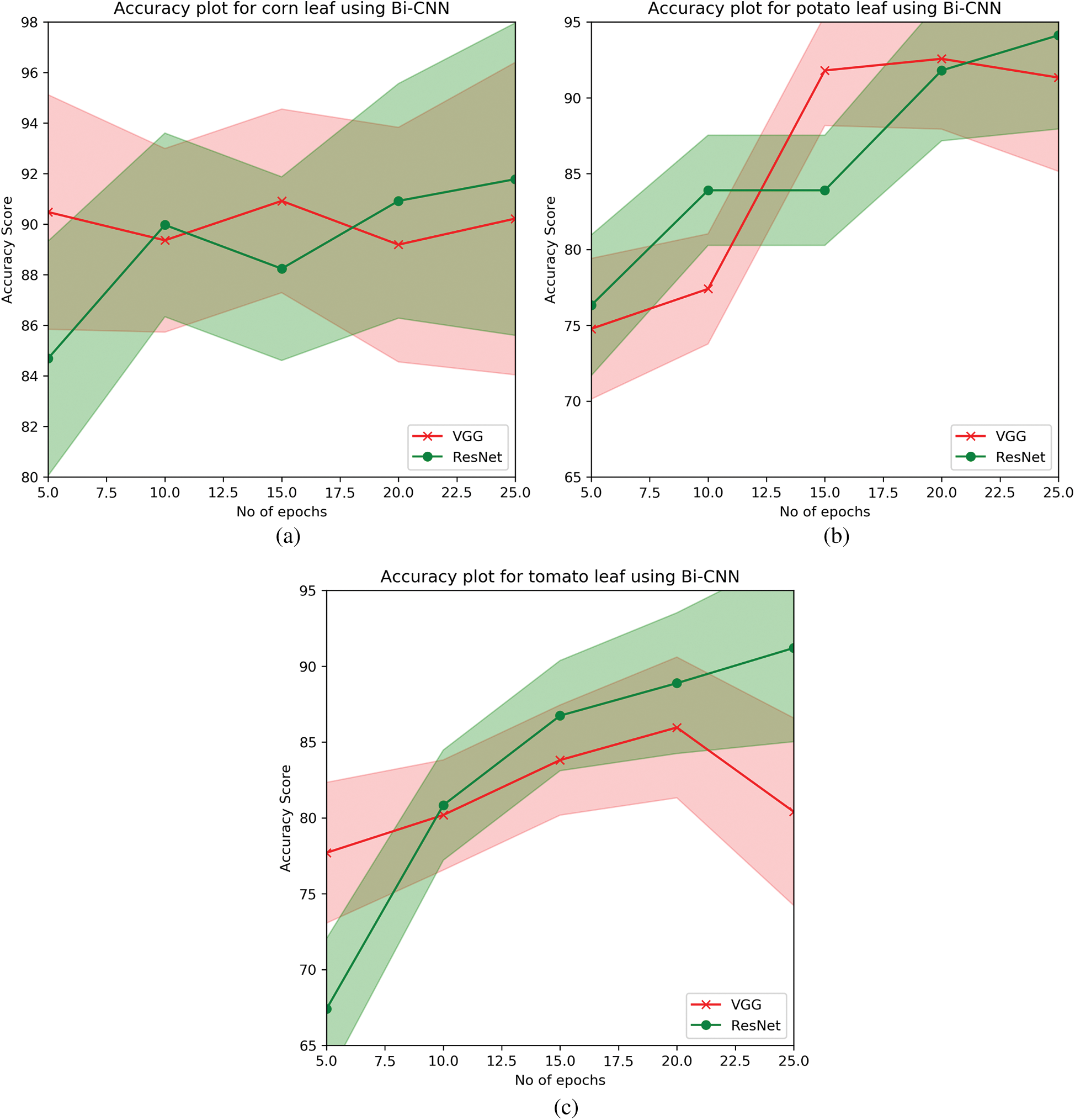
Figure 5: Learning curves of variant models for D2. (a) Accuracy curve of corn (b) Accuracy curve of potato (c) Accuracy curve of tomato
Most of the previous research was held in extracting the features using machine learning methods that do not capture invariances for generic kinds i.e., these models are task-specific and required hand-engineered features. To overcome the problem of extracting features from hand-picked learning mechanisms deep-vision approaches are imparted. Most of the previous work was on developing a convolution neural architecture for extracting features with precise optimization. But, after the evolution of transfer learning [24], many researchers tend to imply these pre-trained weights onto a similar task.
The advantage is, they do not require precise hyperparameter tuning and reduce the computational budget to a greater extent. Hence, these architectures provide pre-trained weights and many kinds of research apply these transfer learning techniques to extract innate bottleneck feature vectors from the given input to classify either using fully connected neural networks or utilizing machine learning classifiers such as SVM, decision trees etc. But, most of the research lack in providing appropriate visual attention to the models an important property of visual recognition task. Providing visual attention to the models can extract fine-grained features containing detailed and precisive information regarding each entity. Further, training or fine-tuning mechanisms should be appropriate for the model to converge fast and generalize well. These problems are addressed by providing a resilient model for capturing detailed invariances and providing 3 level generalizations sets with faster convergence. Further, a Restful-API [25] and mobile application is created for capturing real-time images and classifying them by inserting the proposed model in the back-end. The details about the Restful-API and the application are described in the next section.
The D1 BiCNN’s model performs outrageously even for large test samples providing minute deviation (0.27% for Bi-CNN (sqrt)) from test samples when increased by 5×. Bi-CNN (sqrt) model obtained the highest accuracy 97.88% for 20% test split and CAM activations [33] are visualized to illustrate visual attention.
Next, when tested on, D2, and D3 the model attained the highest accuracy score of 94.98 for 38 classes. When it is evaluated for individual leaf plants with high-class imbalance, ResNet models tend to outperform with an accuracy score of 94.12%, 90.92%, and 91.20% for potato, corn, and tomato plant leaf images respectively from Tab. 4.

7 Restful-API and Mobile Application
In this research, a deep learning model is created and deployed it as a Restful API and connected it to the mobile application for making predictions using an image as input. The REST architectural style is used because of its simplistic interface and modifiability of elements and its ability to adapt to changing needs (even when the application is running) portability of elements by moving data along the program code. It is also scalable for a large number of users. Fig. 6 shows the work-flow of the Restful API that is created. A deep learning model is deployed as REST API which is the most reliable and industrially practiced method for deployment of the deep learning model for making predictions remotely. As you can see in Fig. 6, API accepts base64 encoded image string as input and gives prediction result back in the JSON format. Flask is used for creating the API and also to act as a web server and gateway handler for the input request.
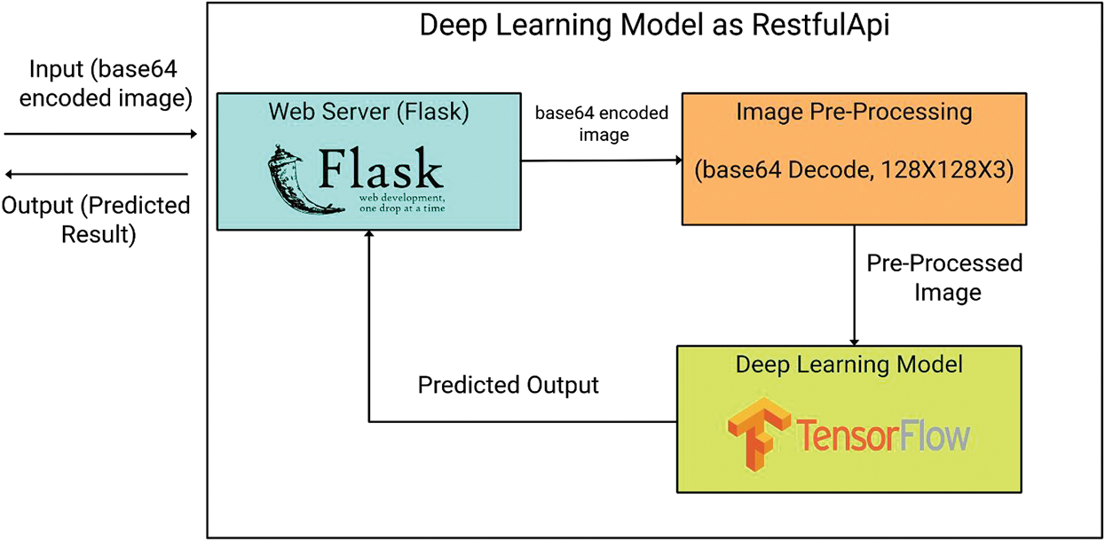
Figure 6: The complete mobile restful-API
In the next stage, the input base64 encoded image string is passed for pre-processing in this stage the base64 encoded image string is decoded and converted back into the image format and also resized the image to 128 × 128 × 3 to be compatible with the model. After the fulfilment of the pre-processing stage, the image is passed as input to the model to make the prediction. The predicted result is passed as output in JSON format. The whole process is wrapped in a single function in API which accepts the base64 encoded image string and outputs the predicted result. We connected this API to a mobile application. Where the user can download the app and predict by uploading or by capturing an image through the camera. Fig. 1 show and walk you through different stages and flow of the mobile app. When an image is uploaded or captured it is converted into a base64 encoded image string and passed to the API handler to handle with proper function then the function runs on the server by invoking the model and passing given base64 encoded image string as the input to the function. This working process is carried out by flask framework using gunicorn as a server in the backend. The restapi was deployed on the Heroku platform.3
The advancement in deep learning is leveraging the performance with the increase in size of data. This eventually led to designing an adaptable kernel [34] which would enhance the feature extraction process both for shallow and deep networks. It is observed that, smaller receptive field implied by VGG, a wavelet kernel [35] and Gaussian kernels [36] obliged in improving the quality of features acquired. The advancement in similarity metrics can acquire scalable features [37–42]. Transforming a sequence of redundant pixels using a specific similarity measure [43–46] is challenging and chosen as future scope for the present work.
This research provides unification with the extension of our conference work [32]. This study is motivated by the human visual cortex in designing an end-to-end trainable neural network named bilinear convolution neural network for plant leaf disease identification and classification. Bi-CNN models are developed for variant data divisions i.e., D1, D2, and D3. These models outperform the existing literature by extracting fine-grained features to provide visual attention through a second-order pooling mechanism. The model attained the highest accuracy score of 94.98% for D3, where 38 variant classes are considered. During this understudy, it is observed that ResNet when implied as a feature extractor outperform the VGG model and provide less computational expense with higher performance. Finally, the model is embedded in a mobile API and released as an opensource. Even with numerous advantages, the methodology didn’t imply 10-fold cross-validation. The 10-fold cross-validation consumes high computational efforts. The proposed second-order pooling generally tend to provide attention only when bottleneck activations which of the same size. Whereas, a new pooling technique has to overcome this disadvantage. The present experiment was carried out on individual leaf images. In future, it is aimed to provide the solution by capturing aerial imaging techniques to extract a bunch of features from clustered plant leaf images with better precision and performance.
Acknowledgement: We are thankful to Jawaharlal Nehru Technological University Hyderabad for sponsoring the fund for publication from TEQIP III under the Collaborative Research Scheme.
Funding Statement: This work was partially supported by the TEQIP-III from Jawaharlal Nehru Technological University Hyderabad, under the Collaborative Research Scheme.
Conflicts of Interest: The authors declare no conflict of interest, financial or otherwise.
1. M. Mortimer, L. G. Ungerleider and K. A. Macko, “Object vision and spatial vision: Two cortical pathways,” Trends in Neurosciences, vol. 6, pp. 414–417, 1983. [Google Scholar]
2. G. U. Leslie and J. V. Haxby, “‘What’ and ‘where’ in the human brain,” Current Opinion in Neurobiology, vol. 4, no. 2, pp. 157–165, 1994. [Google Scholar]
3. S. S. Chouhan, A. Kaul, U. P. Singh and S. Jain, “Bacterial foraging optimization based radial basis function neural network (BRBFNN) for identification and classification of plant leaf diseases: An automatic approach towards plant pathology,” IEEE Access, vol. 6, pp. 8852–8863, 2018. [Google Scholar]
4. K. Aydin, A. S. Keceli, C. Catal, H. Y. Yalic, H. Temucin et al., “Analysis of transfer learning for deep neural network based plant classification models,” Computers and Electronics in Agriculture, vol. 158, pp. 20–29, 2019. [Google Scholar]
5. R. Karthik, M. Hariharan, S. Anand, P. Mathikshara, A. Johnson et al., “Attention embedded residual CNN for disease detection in tomato leaves,” Applied Soft Computing, vol. 86, no. 105933, pp. 1–12, 2020. [Google Scholar]
6. M. P. Sharada, D. P. Hughes and M. Salath “Using deep learning for image-based plant disease detection,” Frontiers in plant science, vol. 7, pp. 1–10, 2016. [Google Scholar]
7. U. S. Pratap, S. S. Chouhan, S. Jain and J. Sanjeev, “Multilayer convolution neural network for the classification of mango leaves infected by anthracnose disease,” IEEE Access, vol. 7, pp. 43721–43729, 2019. [Google Scholar]
8. K. Sandeep, B. Sharma, V. K. Sharma, H. Sharma, J. C. Bansal, “Plant leaf disease identification using exponential spider monkey optimization,” Sustainable computing: Informatics and systems, vol. 28, pp. 1–9, 2018. [Google Scholar]
9. L. Qiaokang, S. Xiang, Y. Hu, G. Coppola, D. Zhang et al., “PD2SE-Net: Computer-assisted plant disease diagnosis and severity estimation network,” Computers and Electronics in Agriculture, vol. 157, pp. 518–529, 2019. [Google Scholar]
10. A. A. Arib, Q. Chen and M. Guo, “Deep learning based classification for paddy pests & diseases recognition,” in Proc. of 2018 Int. Conf. on Mathematics and Artificial Intelligence, 2018. [Google Scholar]
11. I. Monzurul, A. Dinh, K. Wahid and B. Pankaj, “Detection of potato diseases using image segmentation and multiclass support vector machine,” in 2017 IEEE 30th canadian conf. on electrical and computer engineering (CCECEIEEE, pp. 1–4, 2017. [Google Scholar]
12. H. David and M. Salathé, “An open access repository of images on plant health to enable the development of mobile disease diagnostics. arXiv preprint arXiv:1511.08060, 2015. [Google Scholar]
13. S. Karen and A. Zisserman, “Very deep convolutional networks for large-scale image recognition. arXiv preprint arXiv:1409.1556, 2014. [Google Scholar]
14. H. Kaiming, X. Zhang, S. Ren and J. Sun, “Deep residual learning for image recognition,” in Proc.of the IEEE conf. on computer vision and pattern recognition, pp. 770–778, 2016. [Google Scholar]
15. L. T. Yu, A. R. Chowdhury and S. Maji, “Bilinear convolutional neural networks for fine-grained visual recognition,” IEEE transactions on pattern analysis and machine intelligence, vol. 40, no. 6, pp. 1309–1322, 2017. [Google Scholar]
16. I. Sergey and C. Szegedy, “Batch normalization: Accelerating deep network training by reducing internal covariate shift,” in Int. conf. on machine learning, PMLR, 2015. [Google Scholar]
17. S. Nitish, G. Hinton, A. Krizhevsky, I. Sutskever and R. Salakhutdinov, “Dropout: a simple way to prevent neural networks from overfitting,” Journal of Machine Learning Research, vol. 15, no. 1, pp. 1929–1958, 2014. [Google Scholar]
18. G. Xavier and Y. Bengio, “Understanding the difficulty of training deep feedforward neural networks,” in Proc. of the thirteenth int. conf. on artificial intelligence and statistics, JMLR Workshop and Conference Proceedings, 2010. [Google Scholar]
19. K. P. Diederik and J. Ba, “Adam: A method for stochastic optimization,” arXiv preprint arXiv:1412.6980, 2014. [Google Scholar]
20. S. L. Samuel, P. J. Kindermans, C. Ying and Q. V. Le, “Don't decay the learning rate, increase the batch size,” arXiv preprint arXiv:1711.00489, 2017. [Google Scholar]
21. B. Léon, “Stochastic gradient descent tricks,” Neural networks: Tricks of the trade. Berlin, Heidelberg: Springer, pp. 421–436, 2012. [Google Scholar]
22. A. Martín, A. Agarwal, P. Barham, E. Brevdo, Z. Chen et al., “Tensorflow: Large-scale machine learning on heterogeneous distributed systems,” arXiv preprint arXiv:1603.04467, 2016. [Google Scholar]
23. F. Tom, “An introduction to ROC analysis,” Pattern Recognition Letters, vol. 27, no. 8, pp. 861–874, 2006. [Google Scholar]
24. P. S. Jialin and Q. Yang, “A survey on transfer learning,” IEEE Transactions on Knowledge and Data Engineering, vol. 22, no. 10, pp. 1345–1359, 2009. [Google Scholar]
25. R. T. Fielding, Architectural styles and the design of network-based software architectures, vol. 7. Irvine University of California, Irvine, 2000. [Google Scholar]
26. C. C. Albert, A. Luvisi, L. D. Bellis and Y. Ampatzidis, “X-FIDO: An effective application for detecting olive quick decline syndrome with deep learning and data fusion,” Frontiers in plant science, vol. 8, no. 1741, pp. 1–12, 2017. [Google Scholar]
27. A. Marko, M. Karanovic, S. SladojevicA. Anderla and D. Stefanovic, “Solving current limitations of deep learning based approaches for plant disease detection,” Symmetry, vol. 11, no. 17471, pp. 1–21, 2019. [Google Scholar]
28. J. Miaomiao, L. Zhang and Q. Wu, “Automatic grape leaf diseases identification via United Model based on multiple convolutional neural networks,” Information Processing in Agriculture, vol. 7, no. 3, pp. 418–426, 2020. [Google Scholar]
29. K. Aditya, G. Saini, D. Gupta, A. Khanna, S. Tiwari et al., “Seasonal crops disease prediction and classification using deep convolutional encoder network,” Circuits, Systems, and Signal Processing, vol. 39, no. 2, pp. 818–836, 2020. [Google Scholar]
30. T. E. Chebet, L. Yujian, S. Njuki and L. Yingchun. “A comparative study of fine-tuning deep learning models for plant disease identification,” Computers and Electronics in Agriculture, vol. 161, pp. 272–279, 2019. [Google Scholar]
31. S. R. Dammavalam, C. R. Babu, V. S. Kiran, N. Rajasekhar, B. L. Bharadwaj et al., Leaf image classification with the aid of transfer learning: A deep learning approach. Current Chinese Computer Science, 2020. [Google Scholar]
32. C. R. Babu, S. R. Dammavalam, V. S. Kiran, N. Rajasekhar, B. L. Bharadwaj et al., “Deep bi-linear convolution neural network for plant disease identification and classification,” in Advanced Informatics for Computing Research, In press. ICAICR, ISBN: 1393-1394, 2021. [Google Scholar]
33. Z. Bolei, A. Khosla, A. Lapedriza, A. Oliva and A. Torralba, “Learning deep features for discriminative localization,” in Proc. of the IEEE conf. on computer vision and pattern recognition, pp. 2921–2929, 2016. [Google Scholar]
34. C. Youngmin and L. K. Saul, “Kernel methods for deep learning,” in Proc. of the 22nd Int. Conf. on Neural Information Processing Systems, pp. 342–350, 2009. [Google Scholar]
35. H. Huaibo, R. He, Z. Sun and T. Tan, “Wavelet-srnet: A wavelet-based cnn for multi-scale face super resolution,” in Proc. of the IEEE Int. Conf. on Computer Vision, pp. 1689–1697, 2017. [Google Scholar]
36. T. Meng, A. Djelouah, F. Perazzi, Y. Boykov and C. Schroers, “Normalized cut loss for weakly-supervised cnn segmentation,” in Proc. of the IEEE conf. on computer vision and pattern recognition, pp. 1818–1827, 2018. [Google Scholar]
37. R. Vangipuram, R. K. Gunupudi, V. K. Puligadda and J. Vinjamuri, “A machine learning approach for imputation and anomaly detection in IoT environment,” Expert Systems, vol. 37, no. 5, pp. 1–16, 2020. [Google Scholar]
38. S. Aljawarneh and R. Vangipuram, “GARUDA: Gaussian dissimilarity measure for feature representation and anomaly detection in Internet of things,” Journal of Super Computing, Springer, vol. 76, pp. 4376–4413, 2020. [Google Scholar]
39. S. Aljawarneh, R. Vangipuram and A. Cheruvu, “Nirnayam: fusion of iterative rule based decisions to build decision trees for efficient classification,” in Proc. of the 5th Int. Conf. on Engineering and MIS (ICEMIS '19Association for Computing Machinery, New York, NY, USA, pp. 1–7, 2019. [Google Scholar]
40. S. Aljawarneh, V. Radhakrishna and G. S. Reddy, “Mantra: A novel imputation measure for disease classification and prediction,” in Proc. of the First Int. Conf. on Data Science, E-learning and Information Systems (DATA '18Association for Computing Machinery, New York, NY, USA, pp. 1–5, 2018. [Google Scholar]
41. V. Radhakrishna, P. V. Kumar and V. Janaki, “SRIHASS - A similarity measure for discovery of hidden time profiled temporal associations,” Multimed Tools Applications, Elsevier, vol. 77, pp. 17643–17692, 2018. [Google Scholar]
42. V. Radhakrishna, P. V. Kumar and V. Janaki, “Krishna Sudarsana: A z-space similarity measure,” in Proc. of the Fourth Int. Conf. on Engineering & MIS, 2018 (ICEMIS’18Association for Computing Machinery, New York, NY, USA, pp. 1–4, 2018. [Google Scholar]
43. V. Radhakrishna, S. A. Aljawarneh and P. V. Kumar, “ASTRA - A novel interest measure for unearthing latent temporal associations and trends through extending basic gaussian membership function,” Multimedia Tools and Applications, vol. 78, pp. 4217–4265, 2019. [Google Scholar]
44. V. Radhakrishna, S. A. Aljawarneh, P. V. Kumar and V. Janaki, “A novel fuzzy similarity measure and prevalence estimation approach for similarity profiled temporal association pattern mining,” Future Generation Computer Systems, vol. 83, pp. 582–595, 2018. [Google Scholar]
45. V. Radhakrishna, S. A. Aljawarneh, P. V. Kumar and K. R. Choo, “A novel fuzzy gaussian-based dissimilarity measure for discovering similarity temporal association patterns,” Soft Computing, vol. 22, pp. 1903–1919, 2018. [Google Scholar]
46. R. Vangipuram, P. V. Kumar and V. Janaki, “Krishna Sudarsana-A z-space interest measure for mining similarity profiled temporal association patterns,” Foundations of Science, Springer, vol. 25, pp. 1027–1048, 2020. [Google Scholar]
 | This work is licensed under a Creative Commons Attribution 4.0 International License, which permits unrestricted use, distribution, and reproduction in any medium, provided the original work is properly cited. |