Intelligent Automation & Soft Computing DOI:10.32604/iasc.2022.018041
Article

Bayesian Approximation Techniques for the Generalized Inverted Exponential Distribution

Rana A. Bakoban and Maha A. Aldahlan*

Department of Statistics, College of Science, University of Jeddah, Jeddah, Saudi Arabia
*Corresponding Author: Maha A. Aldahlan. Email: maal-dahlan@uj.edu.sa
Received: 22 February 2021; Accepted: 02 May 2021

Abstract: In this article, Bayesian techniques are adopted to estimate the shape parameter of the generalized inverted exponential distribution (GIED) in the case of complete samples. Normal approximation, Lindley’s approximation, and Tierney and Kadane’s approximation are used for deriving Bayesian estimators. Different informative priors are considered, such as Jeffrey’s prior, Quasi prior, modified Jeffrey’s prior, and the extension of Jeffrey’s prior. Non-informative priors are also used, including Gamma prior, Pareto prior, and inverse Levy prior. The Bayesian estimators are derived under the quadratic loss function. Monte Carlo simulations are carried out to make a comparison among estimators based on the mean square error of the estimates. All estimators using normal, Lindley’s, and Tierney and Kadane’s approximation techniques perform consistently since the MSE decreases as the sample size increases. For large samples, estimators based on non-informative priors using normal approximation are usually better than the ones using Lindley’s approximation. Two real data sets in reliability and medicine are applling to the GIED distribution to assess its flexibility. By comparing the estimation results with other generalized models, we prove that estimating this model using Bayesian approximation techniques gives good results for investigating estimation problems. The models compared in this research are generalized inverse Weibull distribution (GIWD), inverse Weibull distribution (IWD), and inverse exponential distribution (IED).

Keywords: Bayesian estimation; generalized inverted exponential distribution; informative and non-informative priors; Lindley’s approximation; Monte Carlo simulation; normal approximation; Tierney and Kadane’s approximation

1  Introduction

Lifetime models are widely used in the statistical inference field. These models are very important in many areas such as engineering, medicine, zoology, and forecasting. The generalized inverted exponential distribution (GIED) is one of the important lifetime models. It is first proposed by Bakoban et al. [1]. GIED is a flexible model because it has various shapes of the hazard function.

The probability density function (PDF) of a two-parameter GIED is

f(x)=(αλx2)exp⁡(−λx)[1−exp⁡(−λx)]α−1,x>0,λ,α>0, (1)

and the cumulative distribution function (CDF) is

F(x)=1−[1−exp⁡(−λx)]α,x>0,λ,α>0, (2)

where α is the shape parameter and λ is the scale parameter.

The GIED distribution has attracted the recent attention of statisticians but has not been discussed in detail in the Bayesian approach. Some authors are interested in this distribution or its generalization [2–8].

On the other hand, others study GIED using Bayesian methods. Ahmed [9] obtains the Bayesian estimators of GIED based on Type II progressive censored samples by applying Lindley’s approximation and importance sampling technique. In addition, Oguntunde et al. [10] discuss Bayesian predictors based on progressive Type-II censoring. Further, Hassan et al. [11] derive the Bayesian estimators based on the Markov Chain Monte Carlo method. Abouammoh et al. [12] study the exponentiated generalized inverse exponential distribution. They derive statistical properties and study applications to real-life data as compared with some other generalized models. Moreover, Singh et al. [13] study Bayesian estimators of reliability function based on upper record value and upper record ranked set sample using Lindley’s approximation. Eraikhuemen et al. [14] discuss Bayesian and maximum likelihood estimation of the shape parameter of the exponential inverse exponential distribution. They use a comparative approach. Bayesian estimation is derived with informative and non-informative priors. In Bayesian analysis, it is well known that Bayesian estimators are usually expressed in an implicit form. Therefore, many approximation procedures are used to evaluate Bayesian estimators. Shawky et al. [15], Singh et al. [16], Sultan et al. [17,18], and Fatima et al. [19] discuss some approximation approaches as the Lindley’s, Tierney and Kadane’s (T-K), and normal approximation methods to compute the Bayesian estimators of the exponentiated Gamma, Marshall-Olkin extended exponential, Kumaraswamy, Topp-Leone, and inverse exponential distributions, respectively. So, in this article, we use normal, Lindley’s, and Tierney and Kadane’s approximation methods to derive Bayesian estimators for the shape parameter of GIED in Sections 2 and 3. The rest of the article is organized as follows. Section 4 studies the simulation and presents numerical results. Section 5 applies the model to real data sets. Finally, Sections 6 and 7 discuss the results and present the conclusion of the study.

2  Bayesian Approximation Methods

The Bayesian estimate of any function of ν, say u(ν), under squared error loss function is

u^(ν)=Eν|x_[u(ν)]=∫0∞u(ν)L(x|ν)π(ν)dν∫0∞L(x|ν)π(ν)dν, (3)

where P(ν|x)=L(x|ν)π(ν) is the posterior function; L(x|ν) and π(ν) are the likelihood function and the prior distribution of ν, respectively. The estimator u^(ν) is also called the posterior mean. The Bayesian method is one of the important estimation methods. Sometimes the posterior distribution contains complicated functions and requires further computation. So, an approximation is needed for the posterior distribution. Thus in this article, we use the following approximation techniques.

2.1 Normal Approximation

When the posterior distribution P(ν|x) has a unimodal symmetric curve, it could be approximated by a normal distribution centered at the mode, so we can write the approximation as

P(ν|x)∼N[ν^,I−1(ν^)], (4)

where I(ν^)=−∂2LogL(ν|x)∂ν2 is the negative Hessian and L(x|ν) is the likelihood function.

2.2 Lindley’s Approximation

Lindley [20] gives an approximation to the following integration ratio

I=∫Ω⁡u(γ)eL(γ)+U(γ)dγ∫Ω⁡eL(γ)+U(γ)dγ, (5)

where L(ν) is the log-likelihood function; u(ν)andU(ν) are arbitrary functions of ν ; Ω represents the value range of ν. Thus the posterior mean, I=E[u(ν)|x], can be evaluated as

I≅u(ν^)+12[u′′(ν^)+2u′(ν^)U′(ν^)]ϕ^2+12[l(3)(ν^)u′(ν^)](ϕ^2)2, (6)

where

l(i)=∂(i)LogL∂ν(i),i=1,2,3,ϕ^2=[−l(2)(ν^)]−1,∂U(ν)∂ν,l=l0=LogL(x|ν), (7)

where L(x|ν) is the likelihood function and π(ν) is the prior distribution.

2.3 Tierney and Kadane’s (T-K) Approximation

For any arbitrary function u(ν) Tierney et al. [21] propose a Laplace form to compute the posterior mean E[u(ν)|x], as

E[u(ν)|x]=∫enη∗(ν)dν∫enη0(ν)dν≅σ^∗enη∗(ν^∗)σ^0enη0(ν^), (8)

nη∗=nη0+Logu(ν), (9)

σ^02=−[∂2∂ν2nη0]−1, (10)

σ^∗2=−[∂2∂ν2nη∗]−1, (11)

where nη0=LogP(ν|x), and P(ν|x) is the posterior distribution.

In the following section, we derive Bayesian estimators for GIED using these approximation methods with different priors.

3  Bayesian Estimators of GIED

In this section, Bayesian approximation techniques are studied for estimating the shape parameter of the generalized inverted exponential distribution based on complete samples. Normal, Lindley’s, and Tierney and Kadane’s approximation methods are used to compute the Bayesian estimators. Also, Bayesian estimators are derived based on squared error loss function for different prior distributions.

Let x=(x1,x2,...,xn) be random samples of size n drawn from a GIED, then by using Eq. (1), the log-likelihood function could be written as

l=LogL(x|α)=nLog(α)+nLog(λ)−αT+∑i=1nLog(xi−2)−λ∑i=1nxi−1−∑i=1nLog(1−e−λ/xi), (12)

where

T=−∑i=1nLog(1−e−λ/xi). (13)

The posterior distribution is obtained by multiplying Eq. (12) with the prior distribution π(α) as

P(α|x)∝lπ(α). (14)

In this article, we choose some informative and non-informative priors, as shown in Tab. 1. In the following subsections, the Bayesian estimators are obtained based on the squared error loss function E(α|x). , which is the posterior mean.

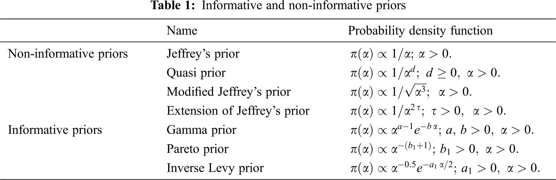
3.1 Bayesian Estimators Using Normal Approximation

In this subsection, we derive Bayesian estimators for GIED using the priors in Tab. 1.

i. Jeffrey’s Prior

According to Eq. (14), the posterior distribution of α is P(α|x)∝αn−1e−αT;α>0, where T is defined in Eq. (13). Then the logarithmic posterior distribution is

LogP(α|x)∝(n−1)Logα−αT. (15)

By taking the first derivative of Eq. (15) concerning α, we get the posterior mode as α^=(n−1)/T. Therefore, the negative of Hessian is I(α^)=T2/(n−1).

The posterior distribution can be approximated as Eq. (3). Thus, for GIED, the posterior distribution can be approximated as P(α|x)∼N[(n−1)/T,(n−1)/T2]. Hence, the Bayesian estimator of α with Jeffrey’s prior using normal approximation is α^=(n−1)/T.

ii. Quasi Prior

The posterior distribution of α is P(α|x)∝αn−de−αT;d≥0,α>0, where T is defined in Eq. (12). Then the logarithmic posterior distribution is

LogP(α|x)∝(n−d)Logα−αT. (16)

By taking the first derivative of Eq. (16) concerning α, we get the posterior mode as α^=(n−d)/T. Therefore, the negative of Hessian is I(α^)=T2/(n−d). The posterior distribution can be approximated as Eq. (3). Thus, for GIED, the posterior distribution can be approximated as P(α|x)∼N[(n−d)/T,(n−d)/T2]. Hence, the Bayesian estimator of α with Quasi prior using normal approximation is α^=(n−d)/T.

iii. Modified Jeffrey’s Prior

The posterior distribution of α is P(α|x)∝αn−3/2e−αT;α>0, where T is defined in Eq. (12). Then the logarithmic posterior distribution is

LogP(α|x)∝(n−3/2)Logα−αT. (17)

By taking the first derivative of Eq. (17) concerning α, we get the posterior mode as α^=(n−3/2)/T. Therefore, the negative of Hessian is I(α^)=T2/(n−3/2).

The posterior distribution can be approximated as Eq. (3). Thus, for GIED, the posterior distribution can be approximated as P(α|x)∼N[(n−1.5)/T,(n−1.5)/T2]. Hence, the Bayesian estimator of α with modified Jeffrey’s prior using normal approximation is α^=(n−1.5)/T.

iv. Extension of Jeffrey’s Prior

The posterior distribution of α is P(α|x)∝αn−2τe−αT;τ>0,α>0, where T is defined in Eq. (12). Then the logarithmic posterior distribution is

LogP(α|x)∝(n−2τ)Logα−αT. (18)

By taking the first derivative of Eq. (18) concerning α, we get the posterior mode as α^=(n−2τ)/T. Therefore, the negative of Hessian is I(α^)=T2/(n−2τ).

The posterior distribution can be approximated as Eq. (3). Thus, for GIED, the posterior distribution can be approximated as P(α|x)∼N[(n−2τ)/T,(n−2τ)/T2]. Hence, the Bayesian estimator of α with the extension of Jeffrey’s prior using normal approximation is α^=(n−2τ)/T.

v. Gamma Prior

The posterior distribution of α is P(α|x)∝αn+a−1e−(b+T)α;a,b>0,α>0, where T is defined in Eq. (12). Then the logarithmic posterior distribution is

LogP(α|x)∝(n+a−1)Logα−(b+T)α. (19)

By taking the first derivative of Eq. (19) concerning α, we get the posterior mode as α^=(n+a−1)/(b+T). Therefore, the negative of Hessian is I(α^)=(b+T)2/(n+a−1).

The posterior distribution can be approximated as Eq. (3). Thus, for GIED, the posterior distribution can be approximated as P(α|x)∼N[(n+a−1)/(b+T),(n+a−1)/(b+T)2]. Hence, the Bayesian estimator of α with Gamma prior using normal approximation is α^=(n+a−1)/(b+T).

vi. Pareto Prior

The posterior distribution of α is P(α|x)∝αn−b1−1e−αT;b1>0,α>0, where T is defined in Eq. (12). Then the logarithmic posterior distribution is

LogP(α|x)∝(n−b−1)Logα−αT. (20)

By taking the first derivative of Eq. (20) concerning α, we get the posterior mode as α^=(n+a−1)/(b+T). Therefore, the negative of Hessian is I(α^)=T2/(n−b−1).

The posterior distribution can be approximated as Eq. (3). Thus, for GIED, the posterior distribution can be approximated as P(α|x)∼N[(n−b−1)/T,(n−b−1)/T2]. Hence, the Bayesian estimator of α with Pareto prior using normal approximation is α^=(n+a−1)/(b+T).

vii. Inverse Levy Prior

The posterior distribution of α is P(α|x)∝αn−1/2e−(T+a1/2)α;a1>0,α>0, where T is defined in Eq. (12). Then the logarithmic posterior distribution is

LogP(α|x)∝(n−1/2)Logα−(T+a1/2)α. (21)

By taking the first derivative of Eq. (21) concerning α, we get the posterior mode as α^=(n−1/2)/(T+a1/2). Therefore, the negative of Hessian is I(α^)=(T+a1/2)2/(n−1/2).

The posterior distribution can be approximated as Eq. (3). Thus, for GIED, the posterior distribution can be approximated as P(α|x)∼N[(n−1/2)/(T+a1/2),(n−1/2)/(T+a1/2)2]. Hence, the Bayesian estimator of α with inverse Levy prior using normal approximation is α^=(n−1/2)/(T+a1/2).

3.2 Bayesian Estimators Using Lindley’s Approximation

With Lindley’s approximation, we can evaluate the posterior mean as Eq. (4). By setting u(α)=α, the posterior mean E[u(α)|x] for GIED can be evaluated as

E(α|x)≅u(α^)+12[u′′(α^)+2u′(α^)U′(α^)]ϕ^2+12[l(3)(α^)u′(α^)](ϕ^2)2. (22)

Using Eq. (12), we obtain LogL(x|α)∝nLogα−αT. Then the maximum likelihood estimator (MLE) of α is α^=n/T. Therefore, the second and third derivatives of the log-likelihood function, as defined in Eq. (7), are

l(2)=∂2l∂α2=−n/α2,andl(2)(α^)=−T2/n, (23)

l(3)=∂3l∂α3=2nα−3,andl(3)(α^)=2T3/n2. (24)

Also,

ϕ2=[−l(2)(α^)]−1=n/T2. (25)

By substituting Eqs. (23), (24), and (25) into Eq. (22), we can evaluate the posterior mean for GIED under different priors as follows.

i. Jeffrey’s Prior

By taking the logarithm of Jeffrey’s prior, we get U(α)≃−Logα,U′(α)=−1/α, and U′(α^)=−T/n.

Then by using Eqs. (22)–(25), we obtain the posterior mean for GIED with Jeffrey’s prior as E[α|x]≅n/T.

ii. Quasi Prior

By taking the logarithm of Quasi prior, we get U(α)≃−dLogα,U′(α)=−d/α, and U′(α^)=−dT/n. Then by using Eqs. (22)–(25), we obtain the posterior mean for GIED with Quasi prior as E[α|x]≅(n−d+1)/T.

iii. Modified Jeffrey’s Prior

By taking the logarithm of modified Jeffrey’s prior, we get U(α)≃−(3/2)Logα,U′(α)=−3/2α, and U′(α^)=−3T/2n. Then by using Eqs. (22)–(25), we obtain the posterior mean for GIED with modified Jeffrey’s prior as E[α|x]≅(2n−1)/2T.

iv. Extension of Jeffrey’s Prior

By taking the logarithm of the extension of Jeffrey’s prior, we get U(α)≃−2τLogα,U′(α)=−2τ/α, and U′(α^)=−2τT/n. Then by using Eqs. (22)–(25), we obtain the posterior mean for GIED with the extension of Jeffrey’s prior as E[α|x]≅(n−2τ+1)/T.

v. Gamma Prior

By taking the logarithm of Gamma prior, we get U(α)≃(a−1)Logα−bα,U′(α)=−b+(a−1)/α, and U′(α^)=−b+(a−1)T/n. Then by using Eqs. (22)–(25), we obtain the posterior mean for GIED with Gamma prior as E[α|x]≅n+aT−nbT2.

vi. Pareto Prior

By taking the logarithm of Pareto prior, we get U(α)≃−(b1+1)Logα,U′(α)=−(b1+1)/α, and U′(α^)=−(b1+1)T/n. Then by using Eqs. (22)–(25), we obtain the posterior mean for GIED with Pareto prior as E[α|x]≅n−b1T.

vii. Inverse Levy Prior

By taking the logarithm of inverse Levy prior, we get U(α)≃−(1/2)Logα−a1α/2,U′(α)=−1/2α−a1/2, and U′(α^)=−(T+a1n)/2n.

Then by using Eqs. (22)–(25), we obtain the posterior mean for GIED under inverse Levy prior as E[α|x]≅(2n+1)T−na12T2.

3.3 Bayesian Estimators Using Tierney and Kadane’s Approximation

To obtain the Bayesian estimator for GIED, we evaluate the posterior mean E[u(α)|x] using Tierney and Kadane’s approximation technique as Eq. (6). By setting u(α)=α in Eq. (6), recalling T as defined in Eq. (11), and using the priors in Tab. 1, the Bayesian estimators are derived as follows.

i. Jeffrey’s Prior

Using Eqs. (9)–(11), we get

nη0=(n−1)Logα−αT, σ^02=(n−1)/T2, nη∗=nLogα−αT, α^∗=n/T , and σ^∗2=n/T2. Then the Bayesian estimator for GIED with Jeffrey’s prior is E[α|x]≅nn+0.5e−1T(n−1)n−0.5.

ii. Quasi Prior

Using Eqs. (9)–(11), we get

nη0=(n−d)Logα−αT, σ^02=(n−d)/T2, nη∗=(n−d+1)Logα−αT, α^∗=(n−d+1)/T , and σ^∗2=(n−d+1)/T2. Then the Bayesian estimator for GIED with Quasi prior is E[α|x]≅(n−d+1)n−d+3/2e−1T(n−d)n−d+1/2.

iii. Modified Jeffrey’s Prior

Using Eqs. (9)–(11), we get

nη0=(n−3/2)Logα−αT, σ^02=(n−3/2)/T2, nη∗=(n−1/2)Logα−αT, α^∗=(n−1/2)/T , and σ^∗2=(n−1/2)/T2. Then the Bayesian estimator for GIED with modified Jeffrey’s prior is E[α|x]≅(n−1/2)ne−1T(n−3/2)n−1.

iv. Extension of Jeffrey’s Prior

Using Eqs. (9)–(11), we get

nη0=(n−2τ)Logα−αT, σ^02=(n−2τ)/T2, nη∗=(n−2τ+1)Logα−αT, α^∗=(n−2τ+1)/T , and σ^∗2=(n−2τ+1)/T2. Then the Bayesian estimator for GIED with the extension of Jeffrey’s prior is E[α|x]≅(n−2τ+1)n−2τ+3/2e−1T(n−2τ)n−2τ+1/2.

v. Gamma Prior

Using Eqs. (9)–(11), we get

nη0=(n+a−1)Logα−(b+T)α, σ^02=(n+a−1)/(b+T)2, nη∗=(n+a)Logα−(b+T)α, α^∗=(n+a)/(b+T) , and σ^∗2=(n+a)/(b+T)2. Then the Bayesian estimator for GIED with Gamma prior is E[α|x]≅(n+a)n+a+1/2e−1(n+a−1)n+a−1/2(b+T).

vi. Pareto Prior

Using Eqs. (9)–(11), we get

nη0=(n−b1−1)Logα−αT, σ^02=(n−b1−1)/T2, nη∗=(n−b1)Logα−αT, α^∗=(n−b1)/T , and σ^∗2=(n−b1)/T2. Then the Bayesian estimator for GIED with Pareto prior is E[α|x]≅(n−b1)n−b1+1/2e−1T(n−b1−1)n−b1−1/2.

vii. Inverse Levy Prior

Using Eqs. (9)–(11), we get

nη0=(n−1/2)Logα−(T+a1/2)α, σ^02=(n−1/2)/(T+a1/2)2, nη∗=(n+1/2)Logα−(T+a1/2)α, α^∗=(n+1/2)/(T+a1/2) , and σ^∗2=(n+1/2)/(T+a1/2)2. Then the Bayesian estimator for GIED with inverse Levy prior is E[α|x]≅(n+1/2)n+1e−1(n−1/2)n(T+a1/2).

4  Simulation and Numerical Results

In this section, a simulation study is conducted to assess the performance of the estimators in the previous section. Mathematica V. 11.0 is used to run a Monte Carlo simulation with 10,000 iterations. Samples of sizes n = 20, 50, 100, and 500 are generated from GIED using the quantile formula x=−λ/Log[1(1−U)1/α],U∼Uniform(0,1), with true values α= 2 and λ= 2. Bayesian estimates are computed using normal, Lindley’s, and Tierney and Kadane’s approximation methods. All estimates are evaluated and tabulated in Tabs. 2–4. Mean square error (MSE) is computed to assess the performance of Bayesian estimates with informative and non-informative priors.

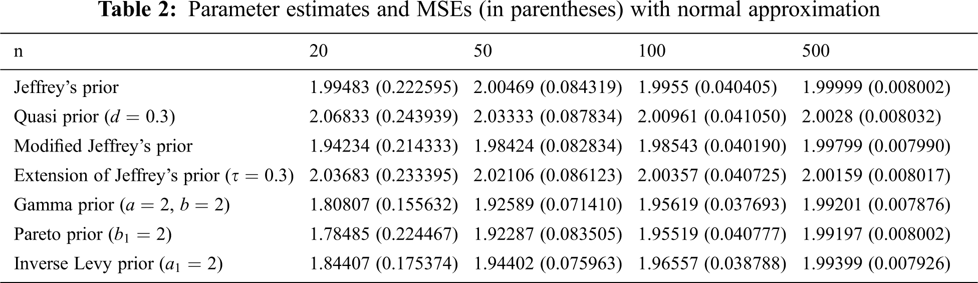
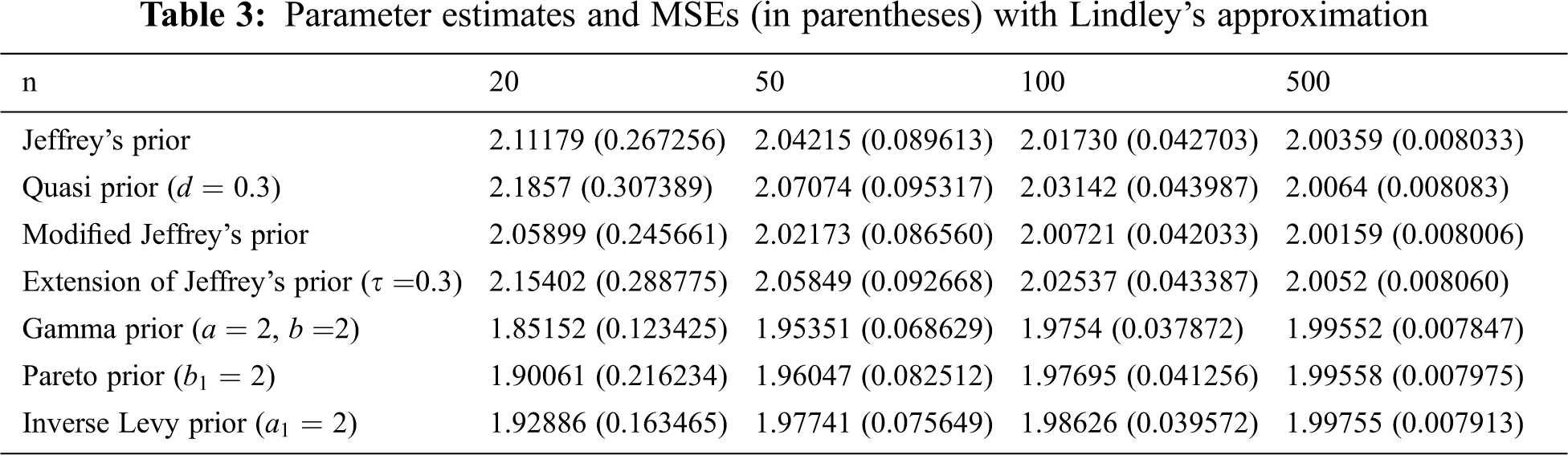
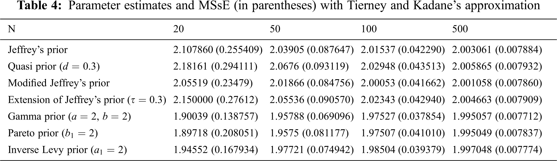
From Tabs. 2–4, we note that all estimators using normal, Lindley’s, and Tierney and Kadane’s approximation techniques perform consistently that the MSE decreases as the sample size increases. In addition, we conclude that the estimator with Gamma prior has the lowest MSE for all techniques. Tierney and Kadane’s technique works more effectively with large samples (n = 100 and 500) than normal and Lindley’s approximations. However, the normal approximation is better than Lindley’s and Tierney and Kadane’s approximations with non-informative priors for n = 20 and 50, and Tierney and Kadane’s approximation is better than Lindley’s approximation in this case. Moreover, estimators under informative priors for n = 20 and 50 using Lindley’s approximation are usually better than normal and Tierney and Kadane’s approximations. For n = 100 and 500, estimators based on non-informative priors using normal approximation are usually better than the ones using Lindley’s approximation. The normal approximation works as well as Lindley’s approximation with informative priors for n = 100, but Lindley’s works better than normal for n = 500 with informative priors.

5  Applications to Real Data

In this section, the GIED distribution is applied to real-life data sets to assess its flexibility over its baseline distribution and some other generalized models. The baseline models are generalized inverse Weibull distribution [22, GIWD], inverse Weibull distribution [23, IWD], and inverse exponential distribution [24, IED]. The fitting performance is evaluated by Kolmogorov-Smirnov (K-S) statistic and some information criteria. A model is the best if it has the lowest Akaike information criteria (AIC), log-likelihood (LL), Bayesian information criterion (BIC), consistent Akaike information criterion (CAIC), and Hannan-Quinn information criterion (HQIC) [25]. The formulas of these criteria are

AIC=−2l(ν^)+2k (26)

BIC=−2l(ν^)+kLogn (27)

CAIC=AIC+2k(k+1)n−k−1 (28)

HQIC=−2l(ν^)+2kLog(Logn) (29)

LL=−2l(ν^) (30)

where l(ν^) denotes the log-likelihood function evaluated at the maximum likelihood estimates ν^, k is the number of parameters, and n is the sample size. The following two case studies illustrate the estimators’ validity in applications.

I. Animal Vaccination Data Set

The first data is the numbers (in thousands) of animals vaccinated against the most widespread epidemic diseases in the 13 regions of Saudi Arabia from 1/1/2020 to 6/30/2020, according to the introduction on the electronic platform (Anaam). This data is downloaded from (https://data.gov.sa/Data/en/dataset/the-numbers-of-animals-vaccinated-against-the-most-widespread-epidemic-diseases).

The statistics of the data set and the performance measures of the models are presented in Tabs. 5 and 6, respectively.

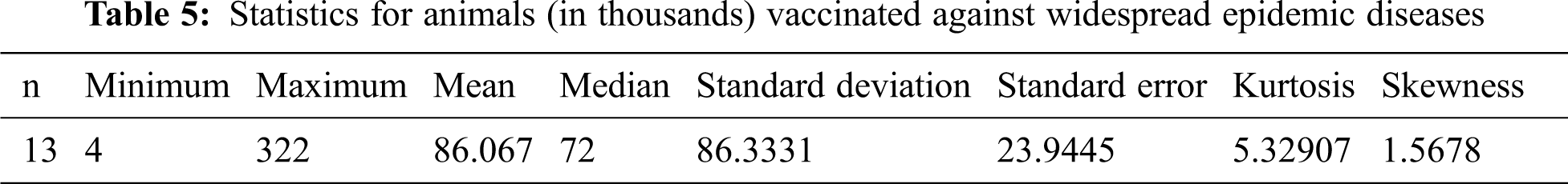
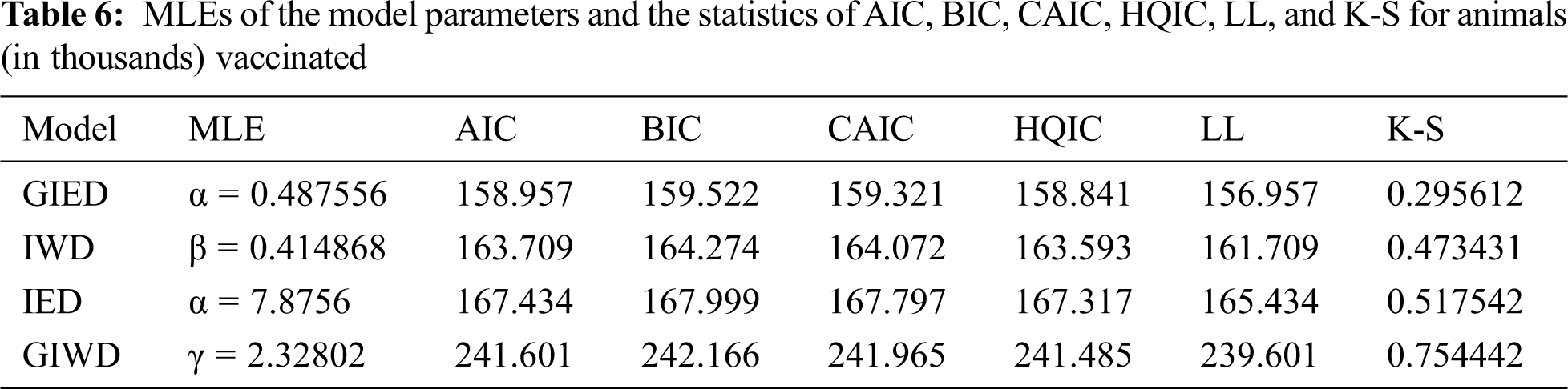
Fig. 1 plots the empirical distribution of the number of animals vaccinated and the estimated CDFs of GIE, IW, IE, and GIW distributions.

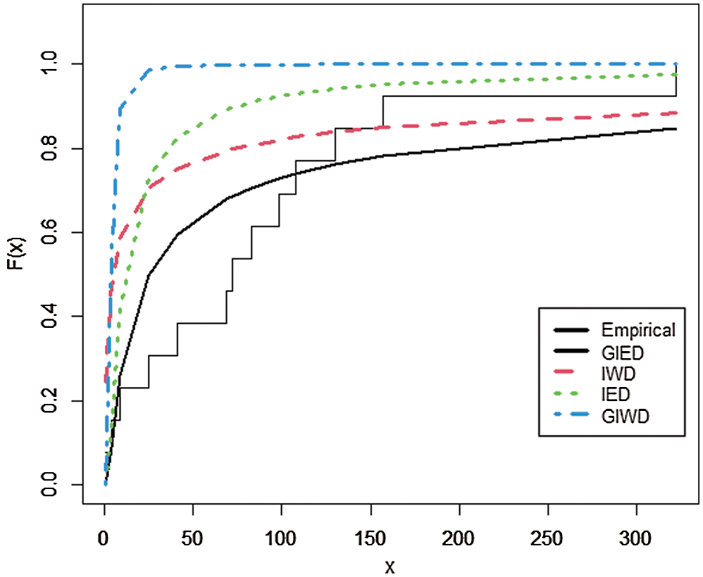
Figure 1: The empirical distribution of the number of animals vaccinated and the estimated CDFs of GIED and other competitive models

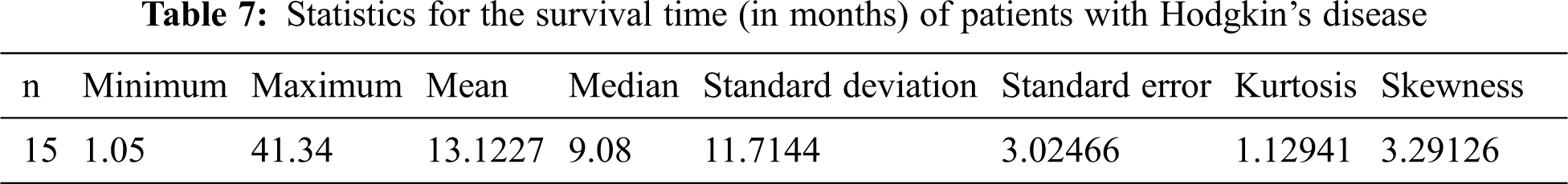
II. Medical Data Set

The second data below shows the survival time (in months) of patients with Hodgkin’s disease and heavy therapy (nitrogen mustards) [26].

The statistics of the data set and the performance measures of the models are presented in Tabs. 7 and 8, respectively.

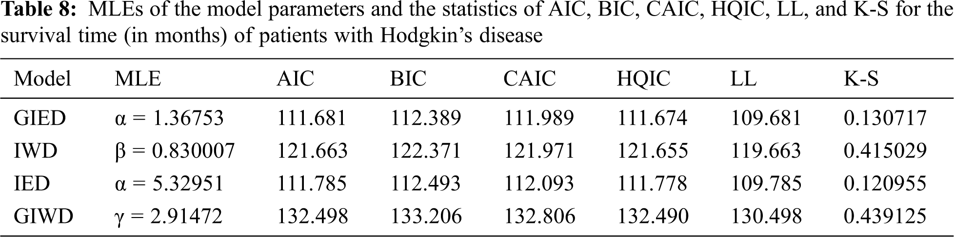
According to the experiments, GIED shows flexibility to real data sets since it has the lowest AIC, BIC, CAIC, HQIC, LL, and K-S as is shown in Tabs. 6 and 8. Our model fits better than the competitive models of IED, IWD, and GIWD. We choose IWD and GIWD as competitive models because GIED is a special case for them. So researchers can use GIED instead of those models. It decreases the amount of computation for estimating and gets better results. On the other hand, GIED shows better fitting performance than its special case IED. Plots in Figs. 1 and 2 show that GIED has the best approximate fitting performance especially for survival time of patients with Hodgkin’s disease.

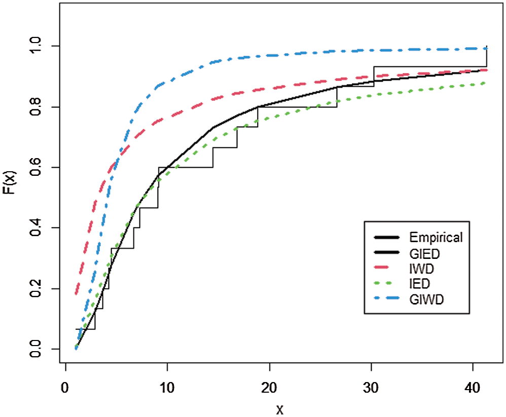
Figure 2: The empirical distribution of survival time of patients and the estimated CDFs of GIED and other competitive models

6  Discussion

It is well known that the Bayesian estimators usually have explicit forms, which is hard for a researcher to code, program, and compute the estimates. Therefore, it is very important to study and compare Bayesian approximation techniques using different priors in statistical inference and especially in Bayesian analysis. These approximations are useful for computing non-closed form estimators, which are very important for reliability analysis. This article presents a comparison among normal, Lindley’s, and Tierney and Kadane’s approximations for Bayesian estimators using seven informative and non-informative priors.

Singh et al. [16] compare Lindley’s, Tierney and Kadane’s, and Markov Chain Monte Carlo (MCMC) methods for Marshall-Olkin extended exponential distribution. Their results show that for n = 20 and 50 with informative priors, Lindley’s works better than Tierney and Kadane’s and MCMC. However, with non-informative priors (Gamma prior), Tierney and Kadane’s has the best estimators.

Fatima et al. [19] compare two techniques: normal and Tierney and Kadane’s for IED. Their results show that normal approximation with the extension of Jeffrey’s prior performs better.

Our results on simulated data show that estimators under informative priors for n = 20 and 50 using Lindley’s approximation are usually better than normal and Tierney and Kadane’s approximations. But with non-informative priors for n = 20 and 50, Tierney and Kadane’s approximation is better than Lindley’s approximation, which agrees with the results of Singh et al. [16].

Moreover, our results in the simulation study show that normal approximation is better than Tierney and Kadane’s approximation with non-informative priors for n = 20 and 50, which agrees with the results of Fatima et al. [19].

Furthermore, in this article, a flexible model, generalized inverted exponential distribution, is used as a lifetime model and applied to two data sets of reliability and medicine. So estimating this model using Bayesian approximation techniques gives good results for investigating estimation problems.

7  Conclusion

In this article, we estimate the shape parameter of GIED using three Bayesian approximation techniques, which are the normal, Lindley’s, and Tierney and Kadane’s approximations. Tierney and Kadane’s works better than the rest of the other methods for large samples. Estimates with informative priors are better than those with non-informative priors. Estimates with Gamma prior are the best among all estimators with the three techniques. This work is a generalization of the inverted exponential distribution studied by Fatima et al. [19].

Acknowledgement: We would like to thank all four reviewers and the academic editor for their interesting comments on the article, greatly improving it in this regard. This work was funded by the University of Jeddah, Saudi Arabia, under grant No (UJ-02-087-DR). The authors, therefore, acknowledge with thanks the University’s technical and financial support. We appreciate the linguistic assistance provided by TopEdit (www.topeditsci.com) during the preparation of this manuscript.

Funding Statement: This work was funded by the University of Jeddah, Saudi Arabia, under grant No (UJ-02-087-DR).

Conflicts of Interest: The authors declare that they have no conflicts of interest to report regarding the present study.

This work is licensed under a Creative Commons Attribution 4.0 International License, which permits unrestricted use, distribution, and reproduction in any medium, provided the original work is properly cited.