Intelligent Automation & Soft Computing DOI:10.32604/iasc.2022.018043
Article

Sine Power Lindley Distribution with Applications

Abdullah M. Almarashi*

Statistics Department, Faculty of Science, King AbdulAziz University, Jeddah, Kingdom of Saudi Arabia
*Corresponding Author: Abdullah M. Almarashi. Email: aalmarashi@kau.edu.sa
Received: 22 February 2021; Accepted: 26 April 2021

Abstract: Sine power Lindley distribution (SPLi), a new distribution with two parameters that extends the Lindley model, is introduced and studied in this paper. The SPLi distribution is more flexible than the power Lindley distribution, and we show that in the application part. The statistical properties of the proposed distribution are calculated, including the quantile function, moments, moment generating function, upper incomplete moment, and lower incomplete moment. Meanwhile, some numerical values of the mean, variance, skewness, and kurtosis of the SPLi distribution are obtained. Besides, the SPLi distribution is evaluated by different measures of entropy such as Rényi entropy, Havrda and Charvat entropy, Arimoto entropy, Arimoto entropy, and Tsallis entropy. Moreover, the maximum likelihood method is exploited to estimate the parameters of the SPLi distribution. The applications of the SPLi distribution to two real data sets illustrate the flexibility of the SPLi distribution, and the superiority of the SPLi distribution over some well-known distributions, including the alpha power transformed Lindley, power Lindley, extended Lindley, Lindley, and inverse Lindley distributions.

Keywords: Sine family; power Lindley model; maximum likelihood method of estimation; applications

1  Introduction

In the last years, many statisticians are attracted by the generated families of distributions, such as Kumaraswamy-G [1], T-X family [2], sine-G [3], Type II half logistic-G [4], exponentiated extended, Muth, odd Frèchet-G [5–7], truncated Cauchy power-G [8], transmuted odd Fréchet-G [9], exponentiated M-G [10], Topp-Leone odd Fréchet-G [11], Sine Topp-Leone-G [12], and generalized truncated Fréchet-G [13].

A new family of continuous distributions referred to as the Sine-G (S-G) family is studied by Kumar et al. [3]. The cumulative distribution function (cdf) of S-G is

F(x;∅)=sin[π2G(x;∅)],x∈R. (1)

where G(x;∅) is the cdf of the baseline model with parameter vector ∅ , and F(x;∅) is the cdf derived by the T-X generator proposed by Kumar et al. [3]. The probability density function (pdf) of the S-G family is

f(x;∅)=π2g(x;∅)cos[π2G(x;∅)],x∈R. (2)

A random variable X has the pdf shown in (2) can be defined as X∼−G(θ,ϕ).

The Lindley (Li) distribution was studied by Lindley et al. [14] and it has the following pdf:

Power Li (PLi) distribution, a new extension of Li distribution, is studied by Ghitany et al. [15]. By exploiting the power transformation X=Tα , this work demonstrated that the PLi distribution is more flexible than the Li and exponential (E) models. The cdf and pdf are

G(x;α,β)=1−(1+βxαβ+1)e−βxα,x>0, (3)

and

g(x;α,β)=αβ2β+1xα−1(1+xα)e−βxα,x>0, (4)

respectively, where β>0 is a scale parameter and α>0 is a shape parameter.

In this paper, an extension of the PLi model is proposed. It is constructed based on the S-G family and the PLi model, and it is called Sine power Lindley (SPLi) distribution.

A non-negative random variable following the SPLi distribution with two parameters β,θ>0 can be constructed by applying (3) and (4) to (1) and (2). The obtained cdf and pdf can be represented as

F(x)=sin[π2(1−(1+βxαβ+1)e−βxα)],α,β>0x>0, (5)

and

f(x)=παβ2xα−12(β+1)(1+xα)e−βxαcos[π2(1−(1+βxαβ+1)e−βxα)],x>0. (6)

The reliability function (survival function) of SPLi distribution is

F¯(x)=1−sin[π2(1−(1+βxαβ+1)e−βxα)]. (7)

The failure rate or hazard rate function (hrf) and reversed hrf for the SPLi are given by

h(x)=παβ2xα−12(β+1)(1+xα)e−βxαcos[π2(1−(1+βxαβ+1)e−βxα)]1−sin[π2(1−(1+βxαβ+1)e−βxα)]. (8)

and

τ(x)=παβ2xα−12(β+1)(1+xα)e−βxαcot[π2(1−(1+βxαβ+1)e−βxα)]. (9)

The plots of the pdf and hrf of the SPLi distribution under various values of parameters are illustrated in Figs. 1 and 2.

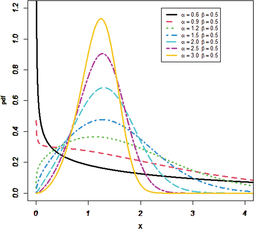
Figure 1: The pdf of the SPLi distribution under various values of parameters

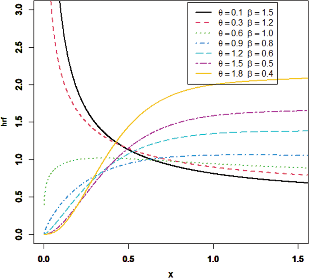
Figure 2: The hrf of the SPLi distribution under various values of parameters

Figs. 1 and 2 present the plots of density and hazard functions of the SPLi distribution under specified values of parameters. It is observed that the pdf of the SPLi distribution is right-skewed, uni-modal, and decreasing. The hrf of the SPLi distribution both increases and decreases.

The rest of this article is arranged as follows: In Section 2, the linear representation of SPLi pdf and cdf are presented. The fundamental properties of the new distribution, including quantile function (qf), moments, moment generating function (MGF), the upper incomplete (UI) moment (UIM), and lower incomplete (LI) moment (LIM), are calculated in Section 3. Different measures of entropy such as Rényi entropy (RE), Havrda and Charvat entropy (HCE), Arimoto entropy (AE), and Tsallis entropy (TE) are derived in Section 4. The parameter estimation following the maximum likelihood (ML) method is studied in Section 5. In Section 6, real data sets are exploited to investigate the potentiality of the SPLi distribution by using some measures of goodness of fits, such as the Akaike Information Criterion (D1), Bayesian Information Criterion (D2), Consistent Akaike Information Criterion (D3), Kolmogorov-Smirnov (D4) statistic. Finally, concluding remarks are presented in Section 7.

2  Important Series

In this section, a linear representation of the pdf is presented to calculate the statistical properties of the SPLi distribution. Eq. (6) can be rewritten as

f(x)=παβ2xα−12(β+1)(1+xα)e−βxαsin[π2(1+βxαβ+1)e−βxα]. (10)

By applying the series of the sine function, i.e., sin[Q]=∑i=0∞(−1)i(2i+1)!Q2i+1 , Eq. (10) can be rewritten as

f(x)=παβ2xα−12(β+1)(1+xα)∑i=0∞(−1)i(π2)2i+1(2i+1)!(1+βxαβ+1)2i+1e−2(i+1)βxα. (11)

By applying the binomial series to Eq. (11), we have

f(x)=∑i,j=0∞(−1)iαβj+2π2i+222i+1(β+1)j+1(2i+1)!(2i+1j)xα(j+1)−1(1+xα)e−2(i+1)βxα. (12)

By applying the binomial expansion to Eq. (12), we have

f(x)=∑i,j=0∞⁡τi,jxα(j+1)−1(1+xα)e−2(i+1)βxα. (13)

where τi,j=(−1)iαβj+2π2i+222i+1(β+1)j+1(2i+1)!(2i+1j).

3  Properties

In this Section, some statistical properties of the SPLi distribution are introduced, such as quantile function (qf), moments, moment generating function (MGF), the upper incomplete (UI) moment (UIM), and lower incomplete (LI) moment (LIM).

3.1 Quantile Function

The qf, i.e., Q(q) =F-1(q), q ∈ (0, 1), is obtained from Eq. (5) and it can be represented as

q=sin[π2(1−(1+βQ(q)αβ+1)e−βQ(q)α)]. (14)

Then,

(1+βQ(q)αβ+1)e−βQ(q)α=1−2πsin−1(q). (15)

By multiplying the two sides of Eq. (15) by (1+β)e−(1+β) , the Lambert equation can be obtained and we have

−(1+β+β(Q(q))α)e−(1+θβ+β(Q(q))α)=−(1+β)e−(1+β){1−2πsin−1(q)}. (16)

Then, the qf is

Q(q)={−1β−1−1βW−1[−(1+β)e−(1+β){1−2πsin−1(q)}]}1/1αα, (17)

where q ∈ (0, 1), and W-1(.) is the negative Lambert W function.

3.2 Moments

The kth moment of X denoted as μk‘ can be derived from Eq. (13) as follows

μk‘=∑i,j=0∞⁡τi,j∫0∞⁡xr+α(j+1)−1(1+xα)e−2(i+1)βxαdx. (18)

Then,

μk‘=∑i,j=0∞⁡τi,j∫0∞⁡(xr+α(j+1)−1+xr+α(j+2)−1)e−2(i+1)βxαdx. (19)

Let y=2(i+1)βxα , then

μk‘=∑i,j=0∞⁡τi,jα[Γ(kα+j+1)(2(i+1)β)kα+j+1+Γ(kα+j+2)(2(i+1)β)kα+j+2]. (20)

Set k=1, and we have E(X)=∑i,j=0∞⁡τi,jα[Γ(1α+j+1)(2(i+1)β)1α+j+1+Γ(1α+j+2)(2(i+1)β)1α+j+2] .

The MGF of X Mx(t) given by Eq. (13) can be represented as

Mx(t)=E(etX)=∑k=0∞tkk!μk‘=∑i,j,k=0∞⁡tkτi,jαk![Γ(kα+j+1)(2(i+1)β)kα+j+1+Γ(kα+j+2)(2(i+1)β)kα+j+2]. (21)

The mth UIM, i.e., ηm(t) , can be calculated as

=∑i,j=0∞⁡τi,jα[Γ(mα+j+1,2(i+1)βtα)(2(i+1)β)mα+j+1+Γ(mα+j+2,2(i+1)βtα)(2(i+1)β)mα+j+2]. (22)

where Γ(m,t)=∫t∞⁡xm−1e−xdx is the UI gamma function.

Similarly, the mth LIM function is given by

=∑i,j=0∞⁡τi,jα[γ(mα+j+1,2(i+1)βtα)(2(i+1)β)mα+j+1+γ(mα+j+2,2(i+1)βtα)(2(i+1)β)mα+j+2], (23)

where γ(m,t)=∫0t⁡xm−1e−xdx is the LI gamma function.

The numerical values of the mean (M), variance (V), skewness (S), and kurtosis (K) of the SPLi distribution are listed in Tabs. 1 and 2.

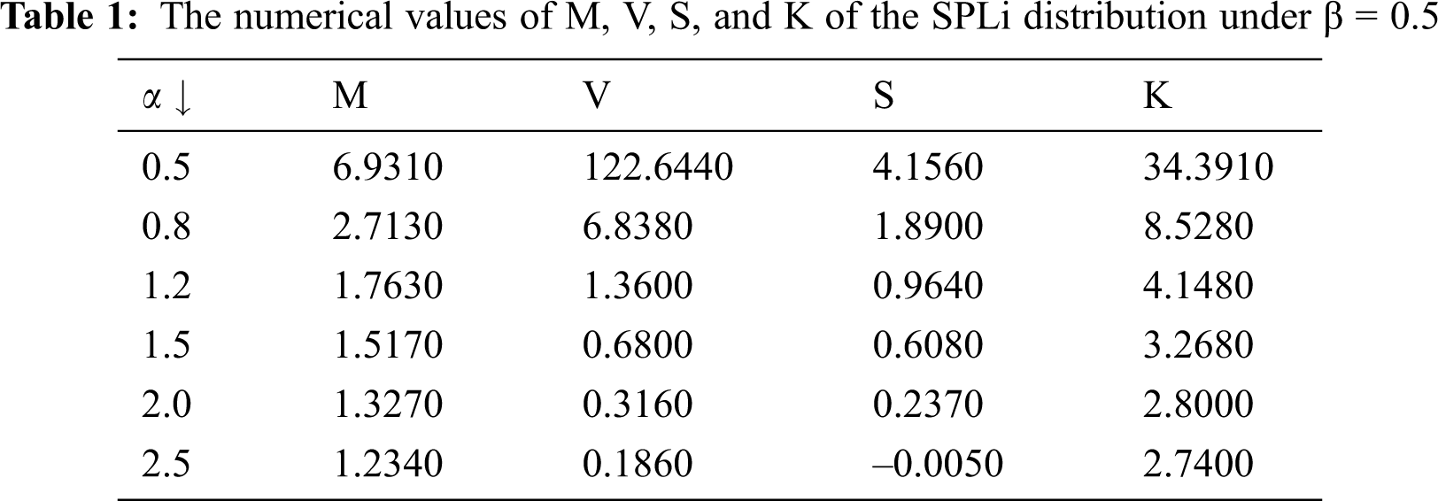
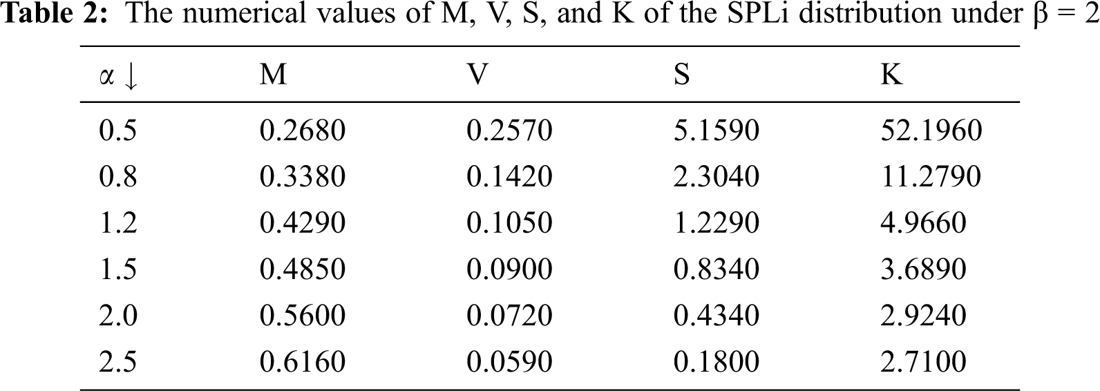
It can be seen from Tabs. 1 and 2 that: when α increases under β = 0.5, the numerical values of M, V, S, and K decrease. Meanwhile, when α increases under β = 2, the numerical values of M increase, but the numerical values of V, S, and K decrease.

4  Different Measures of Entropy

The entropy of the SPLi distribution can be evaluated by different measures, such as Rényi entropy (RE) by [16], Havrda and Charvat entropy (HCE) by Havrda [17], Arimoto entropy (AE) by Arimoto [18], and Tsallis entropy (TE) by Tsallis [19]. These measures of entropy are listed in Tab. 3.

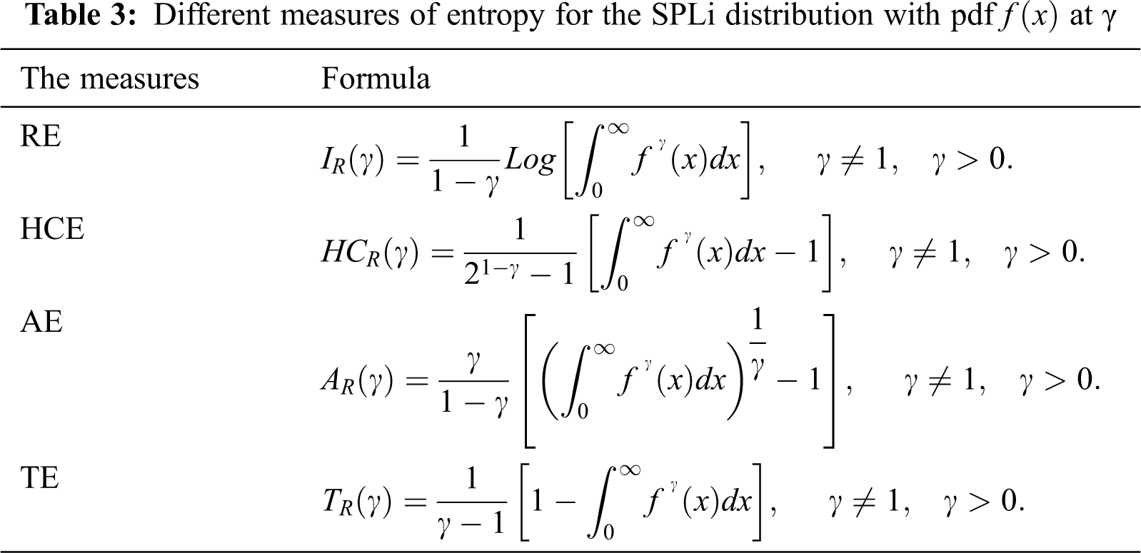
Now, the following integral needs to be calculated:

∫0∞⁡fγ(x)dx=(παβ22(β+1))γ∫0∞⁡xγ(α−1)(1+xα)γe−βγxαcosγ[π2(1−(1+βxαβ+1)e−βxα)]dx. (24)

This integral is very difficult to calculate directly, and it can be solved in a numerical approach. Some of the numerical values of RE, HCE, AE, and TE under the selected values of parameters are given in Tabs. 4–7.

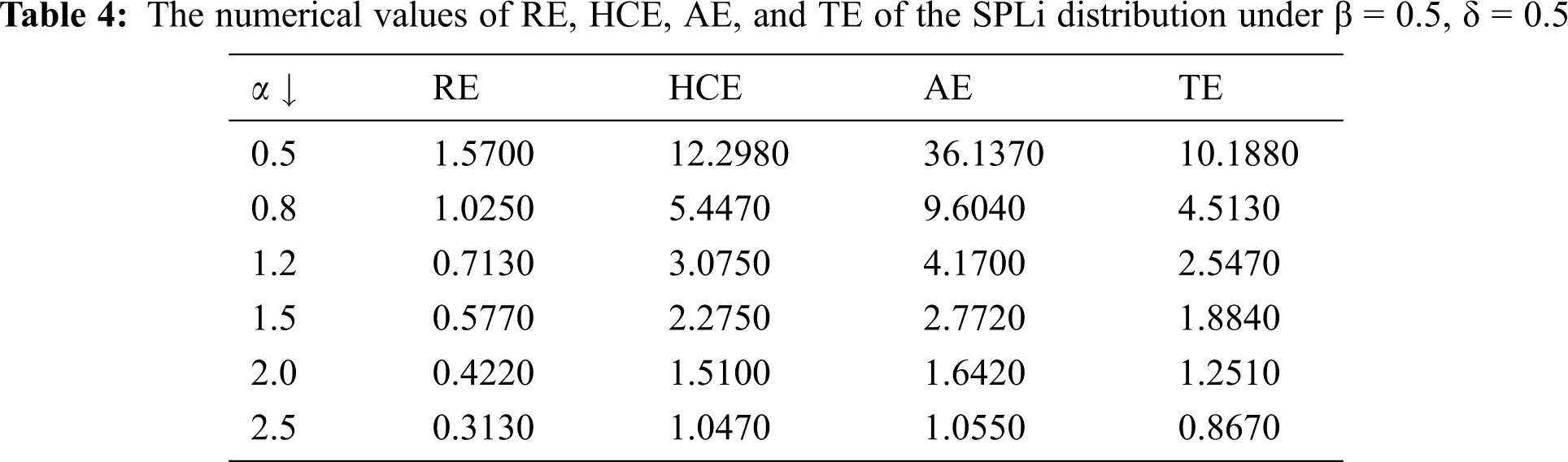
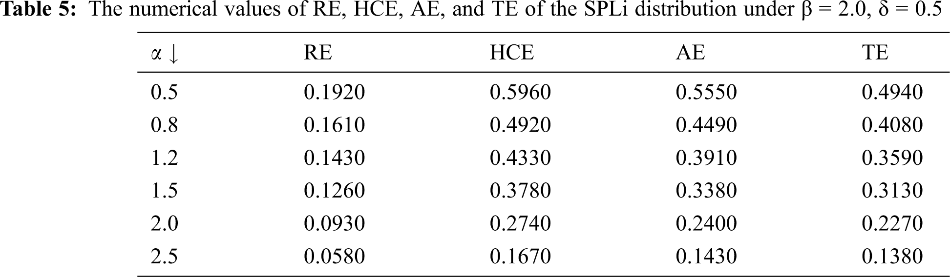
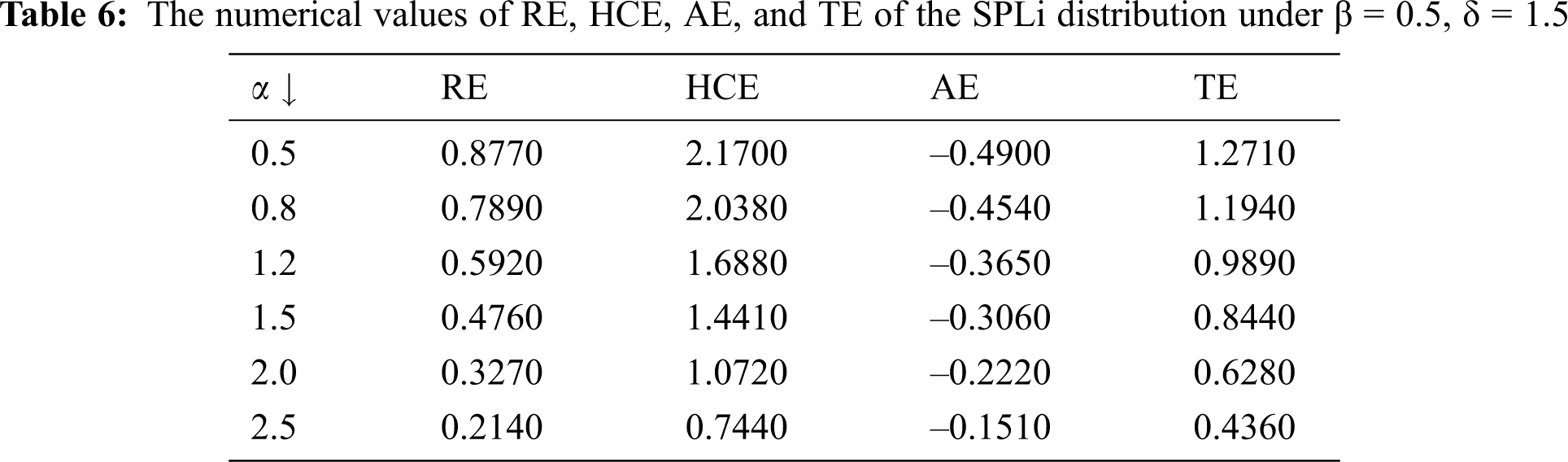
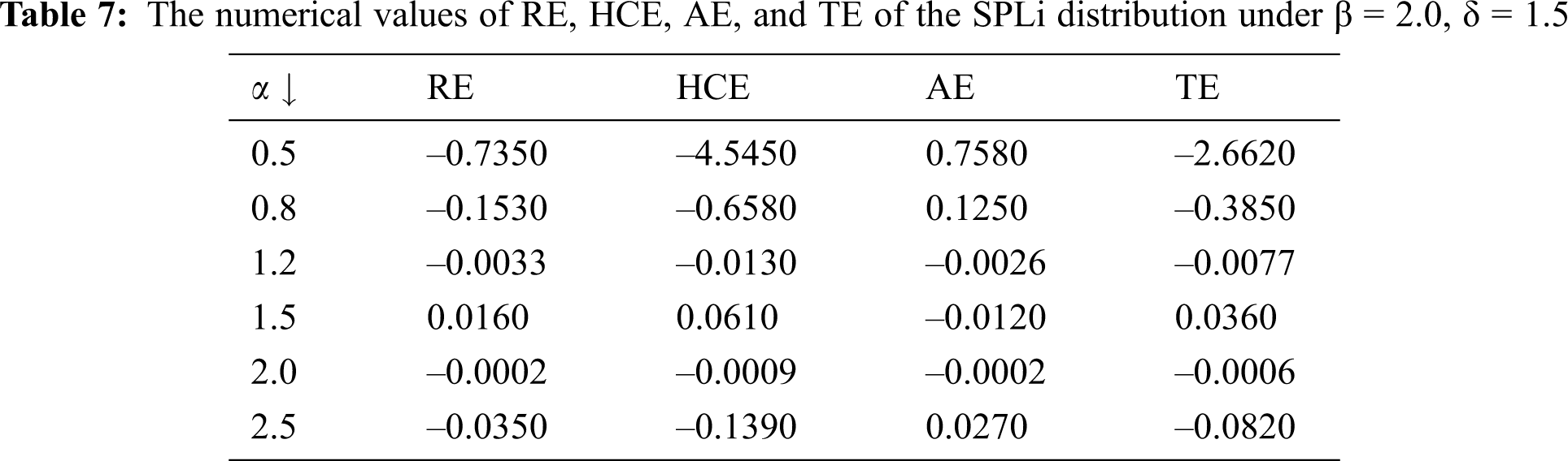
It can be noted from Tabs. 4–7that: When α increases, the numerical values of RE, HCE, AE, and TE decrease. When β increases, the numerical values of RE, HCE, AE, and TE decreases. When δ increases, the numerical values of RE, HCE, AE, and TE decrease.

5  Method of Maximum Likelihood

In this Section, the maximum likelihood (ML) approach is exploited to estimate the parameters α and β of the SPLi distribution. Let x1,x2,...,xn be a random sample of size n from the SPLi distribution with parameters α and β , and the log-likelihood function is

L=nln(πα2)+2nlnβ−nln(β+1)+(α−1)∑i=1n⁡logxi+∑i=1n⁡log((1+(xi)α))−β∑i=1n⁡(xi)α+∑i=1n⁡log[CosZi]. (25)

To calculate the MLE estimation, the partial derivatives of the L by parameters are needed

∂logL∂α=nα+∑i=1n⁡logxi+∑i=1n⁡(xi)αln⁡[xi]1+(xi)α−β∑i=1n⁡(xi)αln⁡[xi]−πβ2∑i=1n⁡(xi)αln⁡[xi]e−β(xi)α(1+β(xi)αβ+1−1β+1)cot[Zi], (26)

and

∂log∂β=2nβ−nβ+1−∑i=1n⁡(xi)α−π2∑i=1n⁡(1+β(xi)αβ+1−1(β+1)2)(xi)αe−β(xi)αcot[Zi], (27)

where Zi=π2(1−(1+β(xi)αβ+1)e−β(xi)α).

6  Modelling

In this section, the SPLi distribution is compared with some other known competitive models to demonstrate its importance in data modeling. Meanwhile, the MLE method is exploited to estimate the parameters of the competitive models. Besides, the measures of goodness-of-fit can be applied to verify the superiority of the SPLi distribution, and D1, D2, D3, and D4 statistics are mainly used.

The fits of the SPLi distribution are compared with that of the distributions including the alpha power transformed Li (APTLi) by Dey et al. [20], PLi, extended Li (EL) by Bakouch et al. [21], Li, and inverse Li (Ili) by Sharma et al. [22]. The first data consists of a sample of 30 failure times of air-conditioning system of an airplane, and the data was introduced by Linhart et al. [23]; the second data consists of 50 failure times of devices which was studied in Aarset [24]. The boxplots and TTT plots of the two data sets are shown in Figs. 3 and 4, respectively. The fitted hrf of the two data sets is shown in Fig. 5, which exhibits an increasing trend. The ML estimates (MLEs), the standard errors (SEs) of the competitive models, and the values of D1, D2, D3, and D4 are presented in Tabs. 8 and 9 for the two data sets.

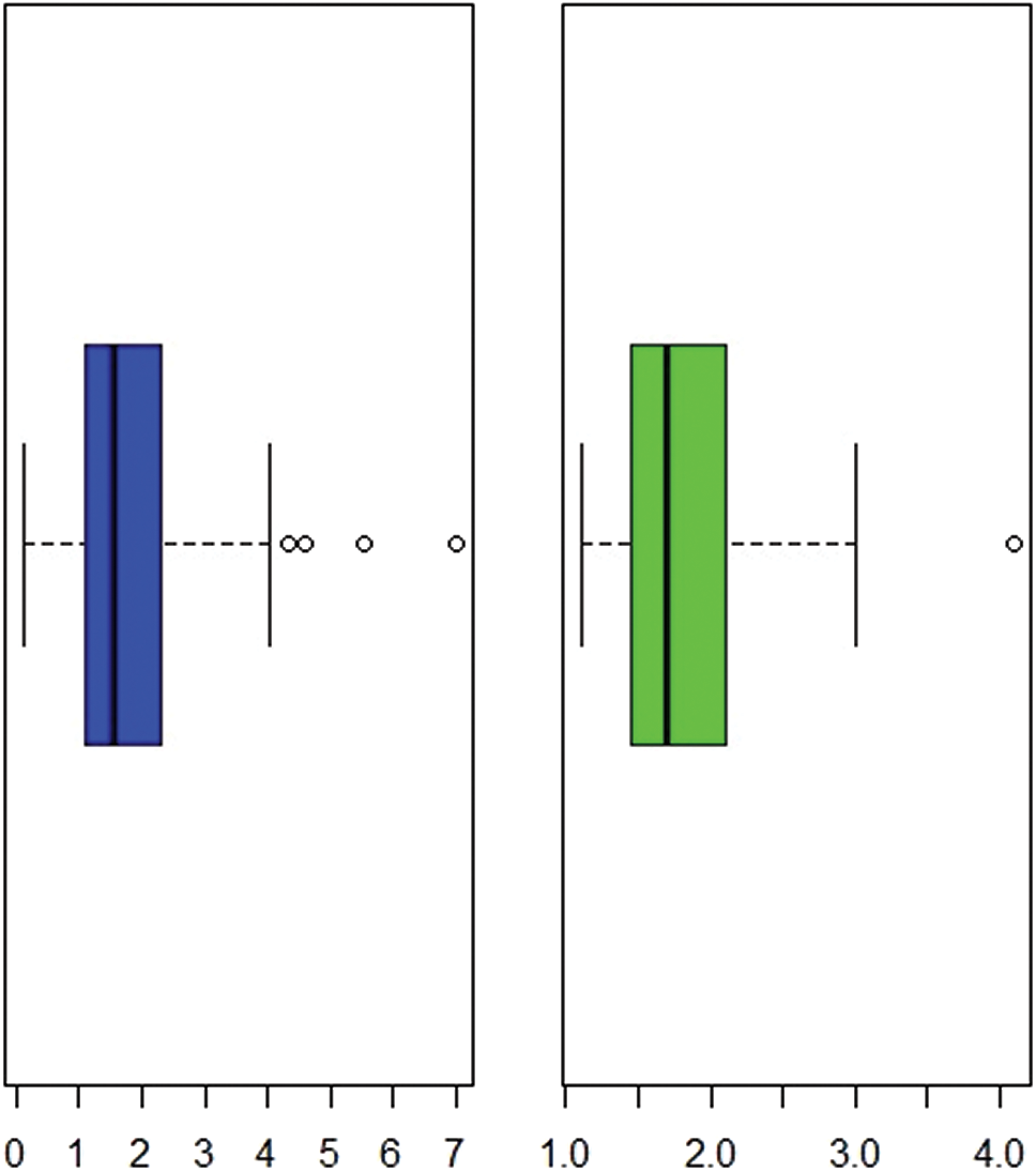
Figure 3: The boxplots of the two data sets

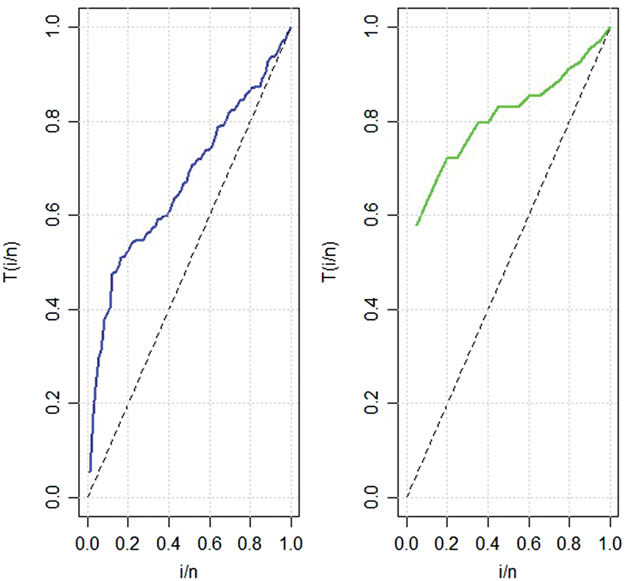
Figure 4: TTT plots of the two data sets

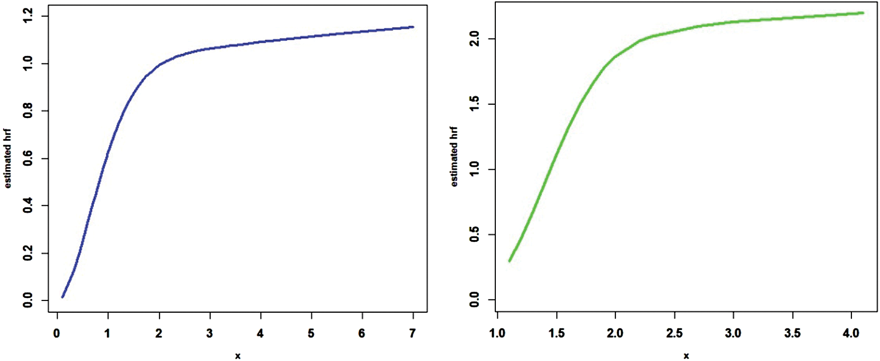
Figure 5: The fitted hrfs of the two data sets

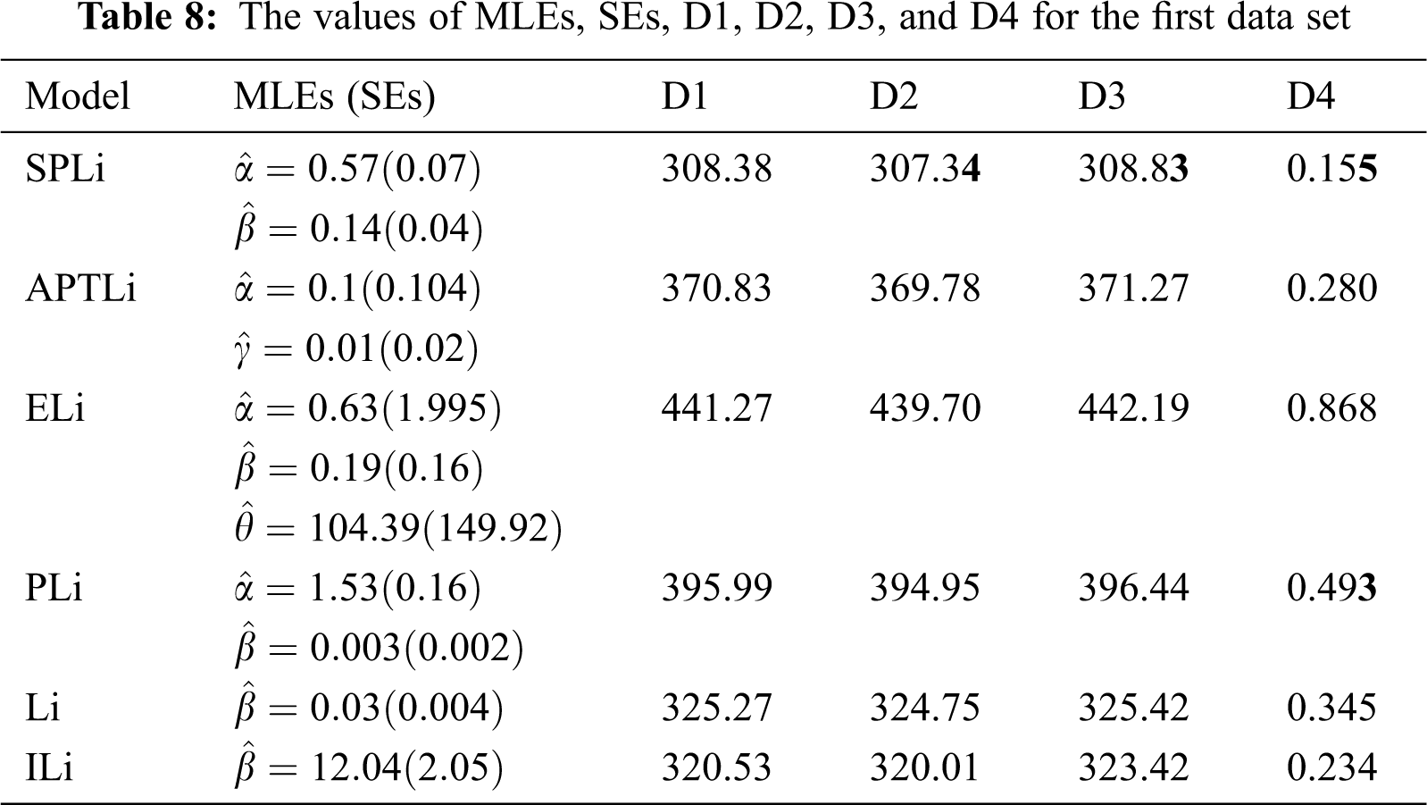
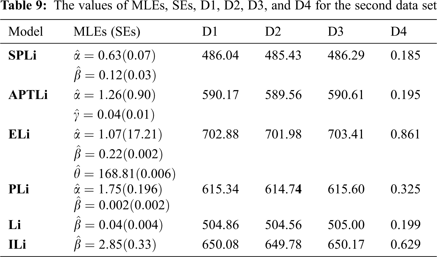
It can be seen from Tabs. 8 and 9 that the SPLi distribution achieves a better fit than the other models for the two data sets. Also, the results in Figs. 6 and 7 indicate the superiority of the SPLi distribution.

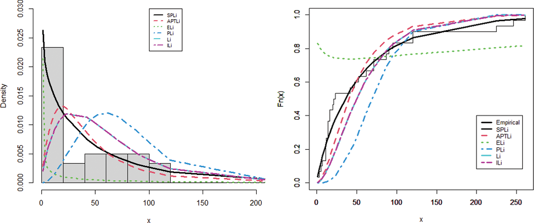
Figure 6: The fitted pdf and fitted cdf of the SPLi for the first data set

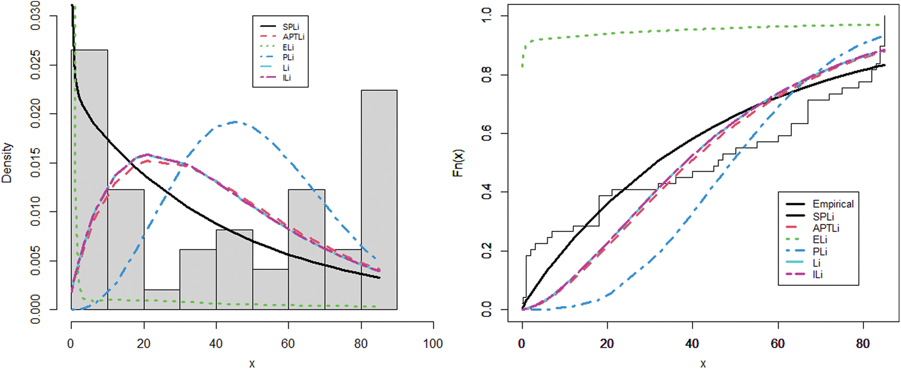
Figure 7: The fitted pdf and fitted cdf of the SPLi for the second data set

7  Concluding Remarks

In this article, a new distribution called Sine power Lindley (SPLi) distribution is introduced. Some statistical properties of the proposed distribution are calculated and discussed, including the quantile function, moments, moment generating function, as well as the upper incomplete moment and lower incomplete moment. Meanwhile, different measures of entropy are studied, including Rényi entropy, Havrda and Charvat entropy, Arimoto entropy, and Tsallis entropy. Besides, the estimation of the model parameters is performed through the ML method. Applications on two real data sets indicate that the proposed SPLi distribution achieves better fits than the other well-known competitive models.

Acknowledgement: I would like to thank all four reviewers and the academic editor for their interesting comments on the article. We appreciate the linguistic assistance provided by TopEdit (www.topeditsci.com) during the preparation of this manuscript.

Funding Statement: The author received no specific funding for this study.

Conflicts of Interest: The author declares no conflict of interest.

This work is licensed under a Creative Commons Attribution 4.0 International License, which permits unrestricted use, distribution, and reproduction in any medium, provided the original work is properly cited.