Intelligent Automation & Soft Computing DOI:10.32604/iasc.2022.018045
Article

A Novel Classification Method with Cubic Spline Interpolation

Husam Ali Abdulmohsin1,*, Hala Bahjat Abdul Wahab2 and Abdul Mohssen Jaber Abdul Hossen3

1Computer Science Department, Faculty of Science, University of Baghdad, Baghdad, Iraq
2Faculty of Computer Science, Technology University, Baghdad, Iraq
3Computer Science Department, Al-Turath University College, Baghdad, Iraq
*Corresponding Author: Husam Ali Abdulmohsin. Email: husam.a@sc.uobaghdad.edu.iq
Received: 23 February 2021; Accepted: 15 May 2021

Abstract: Classification is the last, and usually the most time-consuming step in recognition. Most recently proposed classification algorithms have adopted machine learning (ML) as the main classification approach, regardless of time consumption. This study proposes a statistical feature classification cubic spline interpolation (FC-CSI) algorithm to classify emotions in speech using a curve fitting technique. FC-CSI is utilized in a speech emotion recognition system (SERS). The idea is to sketch the cubic spline interpolation (CSI) for each audio file in a dataset and the mean cubic spline interpolations (MCSIs) representing each emotion in the dataset. CSI interpolation is generated by connecting the features extracted from each file in the feature extraction phase. The MCSI is generated by connecting the mean features of 70% of the files of each emotion in the dataset. Points on the CSI are considered the new generated features. To classify each audio file according to emotion, the Euclidian distance (ED) is found between each CSI and all MCSIs of all emotions in the dataset. Each audio file is classified according to the nearest MCSI to the CSI representing it. The three datasets used in this work are Ryerson Audio-Visual Database of Emotional Speech and Song (RAVDESS), Berlin (Emo-DB), and Surrey Audio-Visual Expressed Emotion (SAVEE). The proposed work shows fast classification and high accuracy of results. The classification accuracy, i.e., the proportion of samples assigned to the correct class, using FC-CSI without feature selection (FS), was 69.08%, 92.52%, and 89.1% with RAVDESS, Emo-DB, and SAVEE, respectively. The results of the proposed method were compared to those of a designed neural network called SER-NN. Comparisons were made with and without FS. FC-CSI outperformed SER-NN on Emo-DB and SAVEE, and underperformed on RAVDESS, without using an FS algorithm. It was noticed from experiments that FC-CSI operated faster than the same system utilizing SER-NN.

Keywords: Classification methods; machine learning; cubic spline interpolation; Euclidean distance; emotional speech dataset; RAVDESS; Emo-DB; SAVEE

1  Introduction

Numeric data are often difficult to analyze, and functions to link the data are hard to find. In 1998, cubic spline interpolation (CSI) was proposed, which connects pairs of data points using unique cubic polynomials, generating a continuous and smooth curve [1]. A spline curve is described by a sequence of polynomials called spline curve segments, and a spline surface is a mosaic of surface patches [2,3].

Interpolation has many applications, all with the purpose of smoothening. The fundamental concept of CSI is based on the engineer’s tool used to draw smooth curves through several points. The spline consists of weights attached to a flat surface. A flexible strip is bent across each of these weights, resulting in a pleasingly smooth curve. The mathematical spline is similar in principle. The points, in this case, are numeric data. The weights are the coefficients of cubic polynomials used to interpolate the data. These coefficients “bend” a line so that it passes through each data point without erratic behavior or breaks in continuity [1]. CSI is used to determine rates of change and cumulative change over an interval. CSI was applied to compute the heat transfer across the thermocline depth of three lakes in the study area of Auchi in Edo State, Nigeria [4]. Spline interpolation methods include linear, quadratic, cubic Hermite, and cubic [5], with different applications. A planning path method based on cubic spline interpolation was proposed to smooth a robot’s moving path [6]. Biodiesel production from waste cooking oil was optimized using CSI and response surface methodology in a mathematical model [7].

We propose an algorithm with third-order CSI curves to classify emotions in three datasets. We are aware of no previous use of CSI in classification, although some research has adopted the idea of this work to discover the wave behavior of an audio signal to classify emotions, using a convolutional neural network (CNN) and not CSI. Related work discovered signal behavior directly from raw data, while FC-CSI works with features extracted from raw data. A network based on time distribution CNN, CNN, and RNN was proposed, without traditional feature extraction to classify emotions, achieving 88.01% classification accuracy on the seven emotions of Emo-DB [8]. A time continuous end-to-end SER prediction system to classify valence and arousal emotions in the RECOLA dataset was proposed [9]. A combination of CNN and LSTM networks learned the representation of a speech signal from raw data. A CNN was proposed to learn and classify emotional features from the spectrogram representation of a speech signal [10], merging feature extraction and classification, with respective classification accuracies of 79.5% and 81.75% on the RAVDESS and IEMOCAP datasets.

CSI has been used in many applications other than classification. Third-order polynomial CSI was used to fit the stress-strain curve of a standardized specimen of SAE 1020 steel hot-rolled flat [11]. Market power points were calculated in different operating conditions and CSI was used to interpolate between them to suggest an appropriate operating condition for a given level of market power [12]. Damage to buildings after a seismic event was assessed by setting boundary conditions based on data from accelerometers at the base and roof and estimating the influence on the other floors [13]. CSI was used in an empirical mode decomposition method to analyze nonstationary and nonlinear signals in communication [14]. Based on its local characteristics in the time domain, the signal was decomposed to a series of complete orthogonal intrinsic mode functions. CSI was used to connect the minimum and maximum signal values to lower and upper envelopes, respectively, and calculate their means. CSI was used to visualize data generated by millions of trajectory frames of molecular dynamic simulations by speeding up the calculation of the atomic density (volumetric map) with a 3D grid from molecular dynamic trajectory data [15].

We propose a classification method utilizing CSI. Classification methods are used in applications such as speech emotion recognition. Regardless of the high accuracy performance achieved by classification algorithms adopting ML methods, their training time is high. We aim to minimize this and propose a classification algorithm that uses cubic spline interpolation, which is a new field in classification research.

The limitation of FC-CSI is the conversion of features from 1D to 2D. To draw a curve on a 2D plane, features must be represented in 2D coordinates, i.e., X and Y. In the proposed algorithm, the feature value is considered the Y-axis, and the sequence of the feature is the X-axis. The distance between features on the X-axis is determined by trial and error, which affects the accuracy, and to find the perfect distance affects system time consumption.

The remainder of this paper is organized as follows. Section 2 explains the proposed algorithm, Section 3 discusses experimental results, and Section 4 relates our conclusions and proposes future work.

2  Proposed Method

We design and implement a classification method. Fig. 1 shows its block diagram. Below, we discuss the blocks in Fig. 1 and explain the data flow of the proposed work.

2.1 Hardware and Software Platform

All experiments were performed using MATLAB R2019a on a computer with an Intel Core I7-8750H CPU @2.2 GHz with 32 GB of RAM and a Windows 10 operating system.

2.2 Datasets

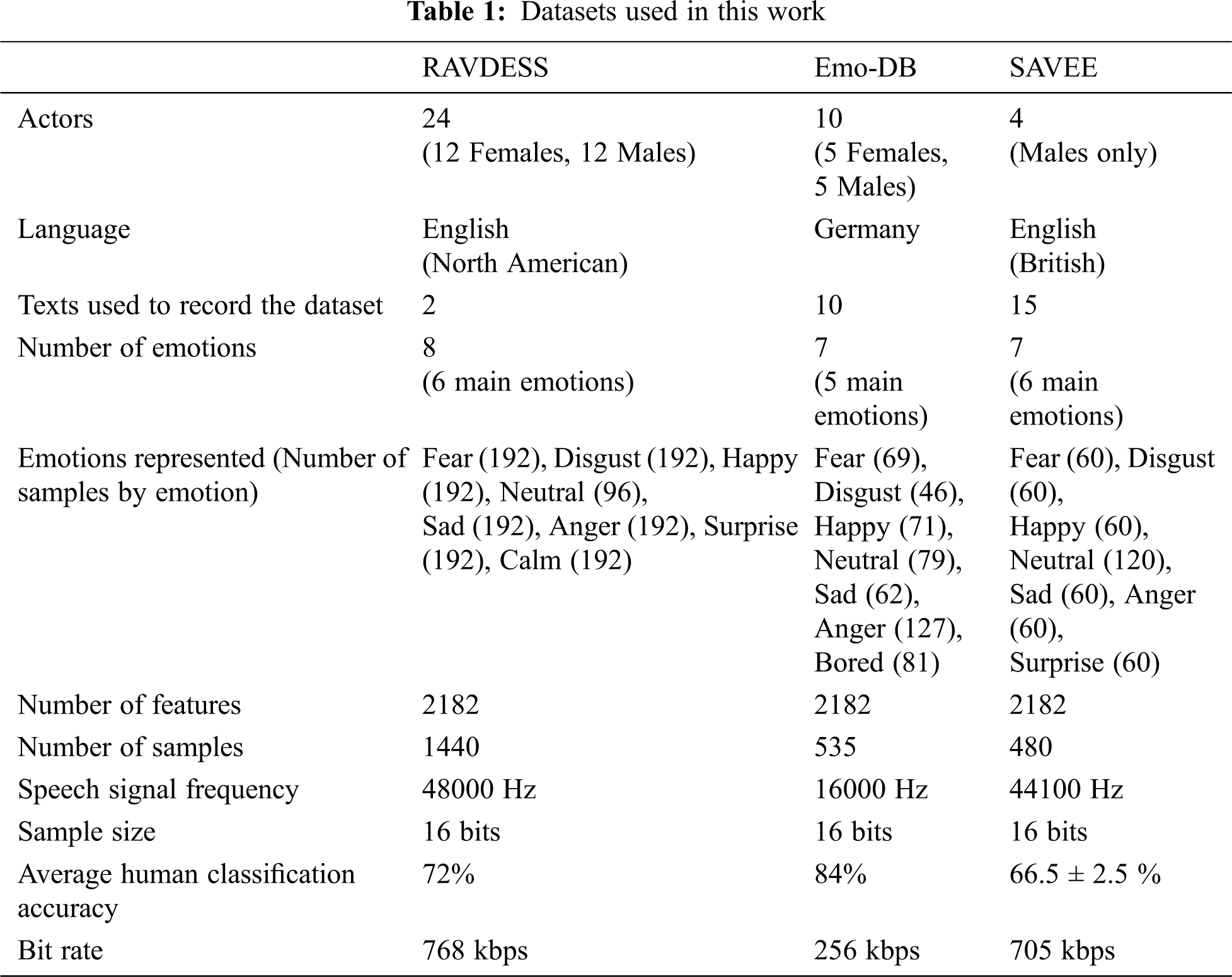
The RAVDESS [16], Emo-DB [17], and SAVEE [18] datasets were used in this work, and were chosen according to the following criteria:

•   Recorded in three frequencies;

•   Representing the main emotions according to Paul Ekman’s definition [19];

•   Two languages were used in recording them;

•   Gender balance was required to be available.

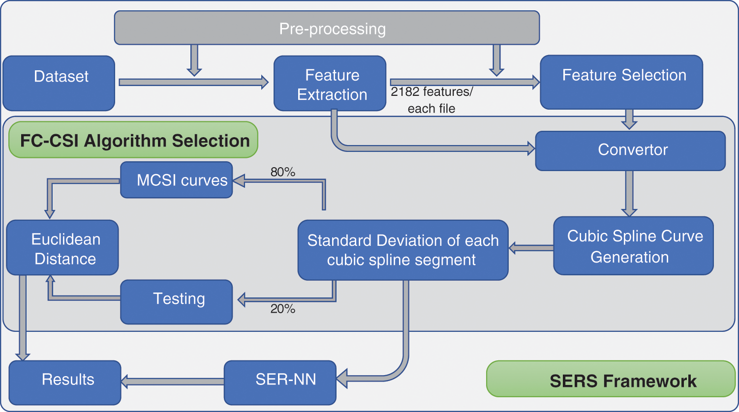
Figure 1: Block diagram of proposed SERS system

The specifications and properties of the datasets are shown in Tab. 1.

2.3 Experimental Setup

Each audio file in a dataset was converted to a one-dimensional vector. Three preprocessing functions were applied to each vector:

1.    All files were grouped according to emotion;

2.    Silent parts at the beginning and end (and not in the middle) of each audio file were removed. This was the first function applied to the data.

3.    Data in each audio vector were normalized between 0 and 100:

xi=(xi−Min)(Max−Min)∗100, (1)

where x is the data read from the audio file; i is the number of values representing the audio file; and Min and Max are the minimum and maximum values, respectively, found in the file. The factor of 100 was discovered through trial and error. This step was applied after feature extraction.

One way to evaluate the performance of the classification method was to compare its results with those of a predefined neural network (NN). We used one hidden layer with 10 nodes. The audio files in each of the three datasets were randomly divided into subsets of 70% for training, 15% for validation, and 15% for testing, and no files were in multiple subsets. The training function used was “trainscg,” the divide function was “dividerand,” and the divide mode was “sample” [20].

2.4 Feature Extraction

The number of features extracted from each audio file was 2182. Fifteen feature types were extracted from each audio file: entropy, zero crossing (ZC), deviation of ZC, energy, deviation of energy, harmonic ratio, Fourier function, Haar, MATLAB fitness function, pitch function, loudness function, Gammatone cepstral coefficient (GTCC) according to time and frequency, and MFCC function according to time and frequency. The deviations (SDs) of these 15 features were calculated using 10 degrees on either side of the mean (including 0.25, 0.5, 0.75, 1, 1.25, 1.5, 1.75, 2, 2.25, and 2.5). The feature extraction function will be called the feature extraction mean deviation (FE-MD) function.

2.5 Converter

This step receives its input from feature extraction and sends its output to cubic spline curve generation, as shown in Fig. 1. It is known that each feature is represented by one numeric value. In order to find the CSI between all features, each feature has to be converted to a two-dimensional coordinate (X and Y). Hence, we assumed the value of the feature to be the Y-axis, and assumed the feature sequence index in the feature vector of each audio file to represent the X-axis of that specific feature. Many experiments were tested, choosing the best spacing between each two features on the X-axis, (i.e., the length of the cubic spline segment), and the best segment length found was 30, which means the first three features will have values of zero, 30, and 60, respectively, on the X-axis, and so on. These are called the control points, or knots, in interpolation [21].

2.6 Cubic Spline Interpolation Generation

Numeric data are commonly difficult to analyze, and a function to successfully link data is hard to find.

In 1998, mathematicians came up with CSI [1]. Fig. 2 shows an example of a single polynomial between control points (xi-1, yi-1) and (xi, yi). A spline curve is composed of a sequence of polynomials called spline curve segments, and a spline surface is a mosaic of surface patches [2,3].

Interpolation algorithms find sets of unique polynomials that form the main spline curve to interpolate all the control points and generate new secured points between them. Changes in control point positions can affect the curvature of the generated polynomials. We chose spline interpolation for three reasons: 1) regardless of polynomial degrees, interpolation error can be small; 2) it avoids Runge’s phenomenon [22,23] because when high-degree polynomials are used, oscillation can occur between points; 3) the generated polynomials serve as a technique to sketch smooth secured curves [24].

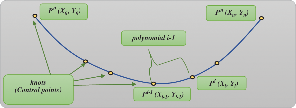
Figure 2: Interpolation with cubic splines between seven points, using flexible rulers bent to follow predefined points (“control points”) in yellow

Interpolation has many applications, and all follow the concept of smoothening [1,21]. We first explain the concept of the degree of a polynomial. A polynomial is a mathematical expression that can be formed from constants and symbols (like x and y), which are also called variables or indeterminants. The constants and variables are connected by means of multiplication, addition, and exponentiation to positive integer powers. A polynomial of a variable (x) can be written as

anxn+an−1xn−1+…+a2x2+a1x1+a0 (2)

where a0 , a1, …, an are constants, and x is the variable (indeterminant). The word “indeterminant” indicates that x represents no specific value, and therefore can take any value. A function that maps the result of substitution with a value is called a polynomial function. Eq. (2) can be written as

∑k=0nakxk (3)

Therefore, a polynomial can be written as either zero or as a sum of a limited number of nonzero terms, each the product of a number (coefficient) and a finite number of variables raised to a positive integer power. The power is called the degree, and the degree of a polynomial is the largest degree among all terms with nonzero coefficients. An example of a cubic polynomial is

−5x3+4x2+1x+7 (4)

The degree of the second term is 2, and the coefficient of the term is +4. The degree of the polynomial is the degree of the highest term, i.e., three.

A third-degree spline is called a cubic spline. Let us assume a cubic spline in the interval x0 ≤ xi ≤ xn is generated by a set of piecewise polynomials si (x). The standard form of the cubic spline is

Ri(x)=ai+bi(x−xi)+ci(x−xi)2+di(x−xi)3, (5)

where i = 1, 2, …, n-1; and n is the number of control points. Hence, n-1 is the number of cubic polynomials that will form the cubic spline interpolation. The first and second derivatives of these n-1 equations are fundamental in cubic spline interpolation methodology, and these are respectively shown as [25]

(6)

Ri′′(x)=2ci+6di(x−xi).0 (7)

From these functions, three matrices can be generated (see Fig. 3), and we can write

Ax=b. (8)

Eq. (5) can be solved to obtain coefficients a, b, c, and d of the cubic spline polynomial [26–29].

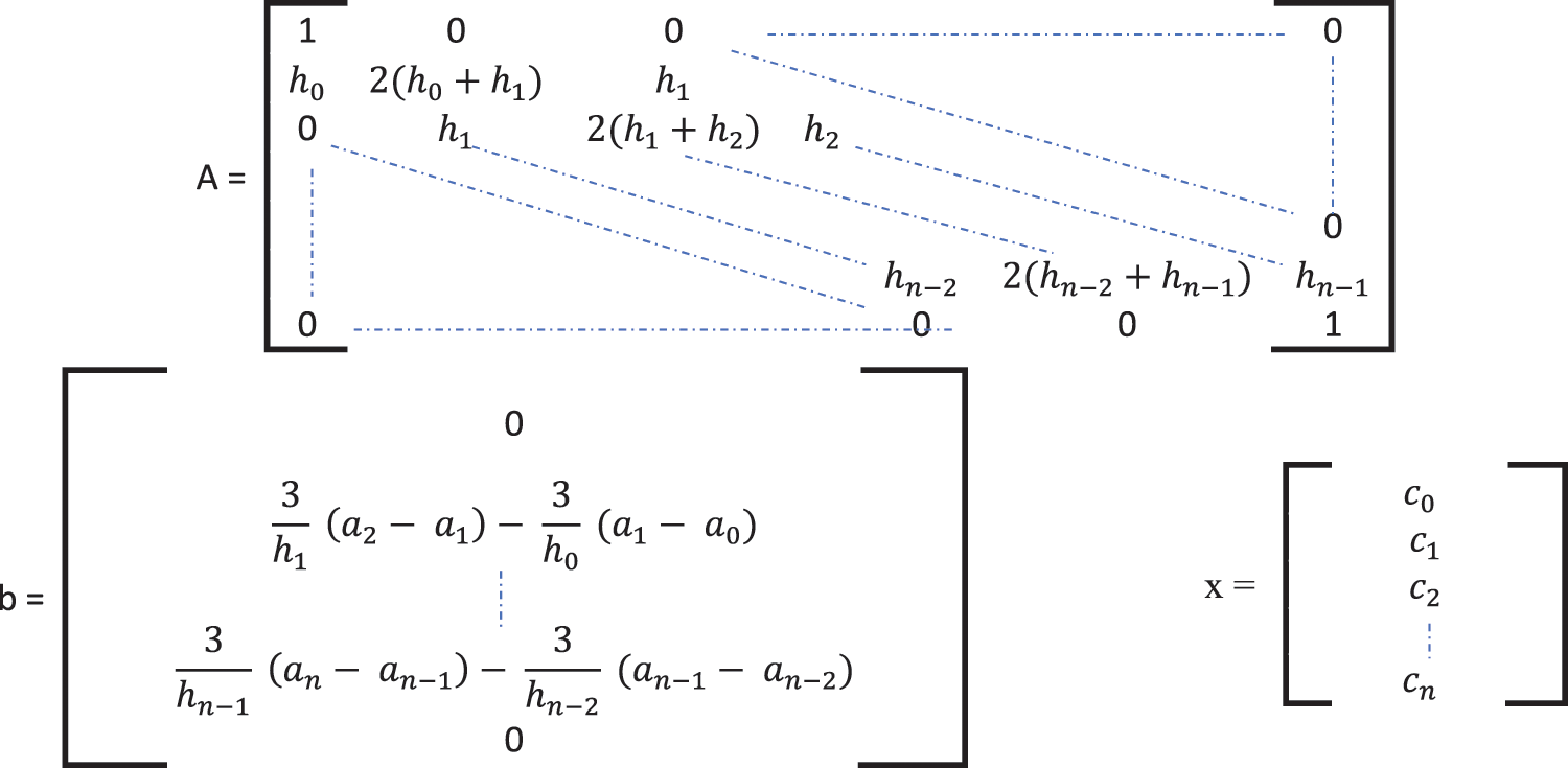
Figure 3: Matrices used to find the four coefficients (a, b, c, and d) of CSI

2.7 Standard Deviations of Cubic Spline Segments

This step generates CSI with equal lengths, so 10 deviation degrees (0.25, 0.5, 0.75, 1, 1.25, 1.5, 1.75, 2 (standard deviation), 2.25, and 2.5) will be found for all points in each polynomial to construct the final spline curve. After this step, CSIs representing all audio files in the dataset will be randomly divided into two parts, 70% to find the MCSI curves and 30% for testing.

2.8 Finding Mean Cubic Spline Interpolation Curves

Each MCSI curve represents a different emotion, so the number of MCSI curves is the number of emotions represented in the dataset, i.e., 8, 7, and 7 for RAVDESS, EMO-DB, and SAVEE, respectively. MCSI is calculated as

MCSI(m)=(nm=1)(x=21820j=1)(∑i=1y(m)CSI(i,j))/length(y(m)), (9)

where m = 1, 2, …, n; n is the number of emotions in the dataset; j = 1, 2, …, x, where x is the number of points forming each CSI representing each audio file; i = ∈ y(m), where vector y(m) stores 70% of the audio files indices randomly selected from each emotion. The feature subset is (fij, fi+1j, fi+2j, …, fnj), where length (y(m)) equals 1152, 428, and 384, for RAVDESS, EMO-DB, and SAVEE, respectively. At the end of this step, m MCSIs will be generated, where m equals the number of emotions. Each MCSI represents a different emotion though a unique curve. The summation will add the same 70% sample from each feature subset, as defined in Tab. 2. The MATLAB code of MCSI generation is shown in Fig. 4.

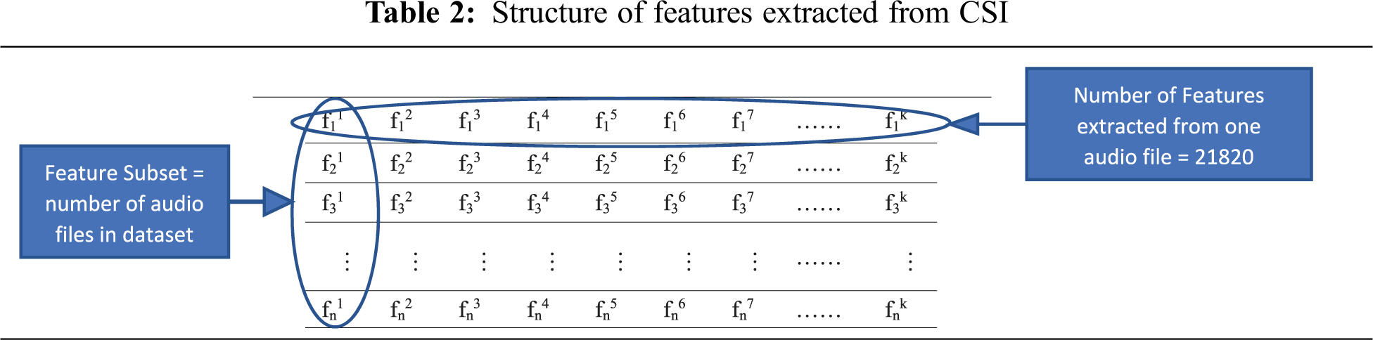
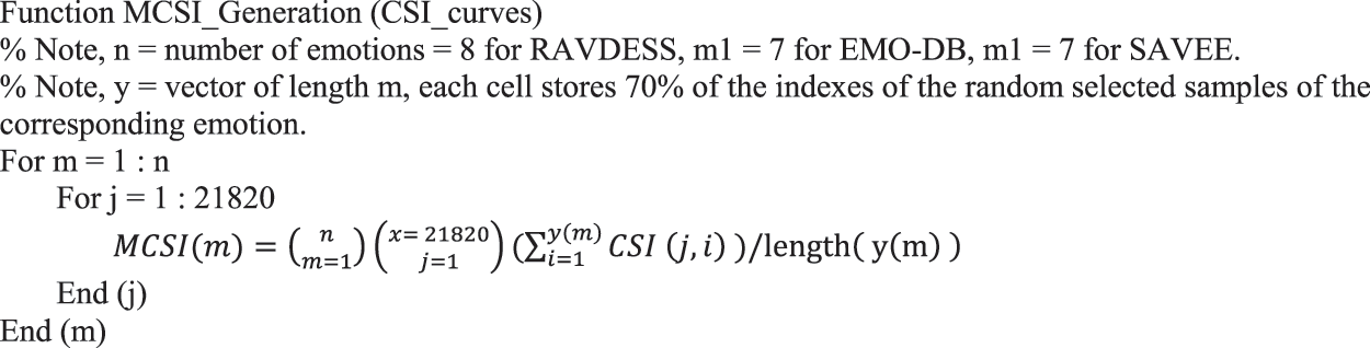
Figure 4: MATLAB code for MCSI generation

2.9 Testing

The audio files in the dataset will be divided into two groups, training and testing. The 70% for training will be used to find the MCSIs, and the remaining 30% of the audio files in the dataset, will be used to test the classification accuracy of the proposed work. This 30% is 432, 160, and 144 audio files for RAVDESS, EMO-DB, and SAVEE, respectively.

2.10 Euclidean Distance

The standard Euclidean distance function is used in this work [30]:

EDnm=∑i=j=1n=21820((Xjm−Xin)2+(Yjm−Yin)2), (10)

where (Xin, Yin) are the coordinates of the CSI samples determined for testing, and (Xjm, Yjm) are the coordinates of the MCSI curve that represents one of the emotions in the dataset. The matrix that will be generated from Eq. (10) and the MATLAB code in Fig. 5 will be an n × m matrix, where n is the number of testing audio samples and m is the number of emotions in the dataset. Each audio sample will be classified according to the closest MCSI to the CSI that represents it.

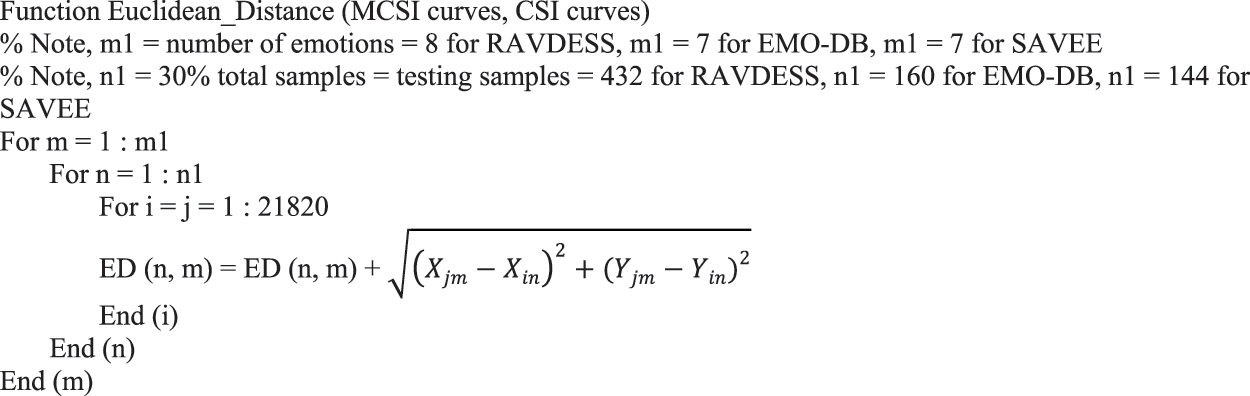
Figure 5: MATLAB code for Euclidean distance function

3  Experimental Results

We analyze the performance of SERS. The best classification accuracy results will be discussed with respect to the fewest features selected. Experiment 1.1 (Exp1.1) and experiment 1.2 (Exp1.2) were respectively performed before and after deploying the pre-designed feature selection t-test fitness (FS-TF) algorithm.

3.1 Experiment 1.1: SERS Performance Analysis Before Deploying Feature Selection Algorithm

Through Exp1.1, the classification performance of SERS is calculated in two different approaches. First, utilizing the FC-CSI algorithm and second through utilizing the SER-NN. Both approaches are implemented without deploying the FS-TF algorithm.

3.1.1 SERS Accuracy Performance

Figs. 6–8 show the classification accuracy results of Exp1.1 after running the FC-CSI classification algorithm. Figs. 9–11 show the classification accuracy results of Exp1.1 after running the SER-NN classification algorithm. Tab. 3 shows the results of Exp1.1 implemented on the 2182 FE-MD features extracted from the RAVDESS, EMO-DB, and SAVEE datasets, without feature selection.

We observe the following after analyzing the results:

•   Results from Exp1.1 show that FC-CSI outperformed SER-NN FC on Emo-DB and SAVEE and underperformed on RAVDESS. This leads to the conclusion that, FC-CSI does not perform well on datasets of low human-accuracy performance.

•   The most misclassified samples are those of the sad and fear emotions in RAVDESS, and neutral, sad, and disgust in SAVEE, which shows the drawback of FC-CSI in recognizing low-amplitude emotions.

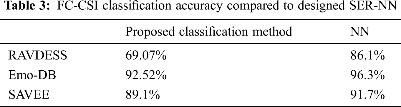
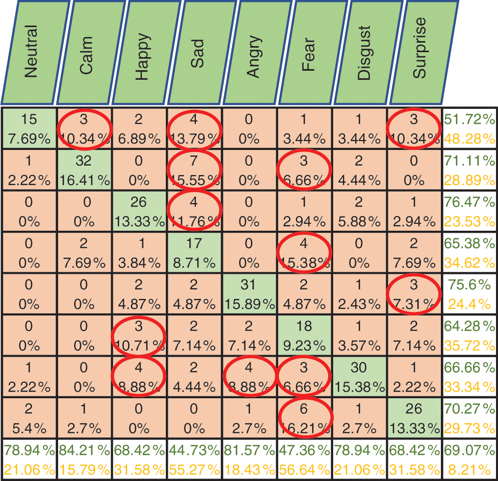
Figure 6: Exp1.1, SERS, FC-CSI, confusion matrix with RAVDESS, without FS

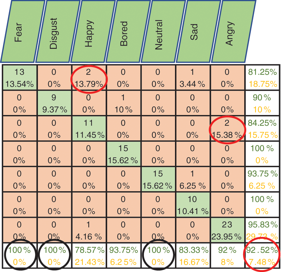
Figure 7: Exp1.1, SERS, FC-CSI, confusion matrix with Emo-DB, without FS

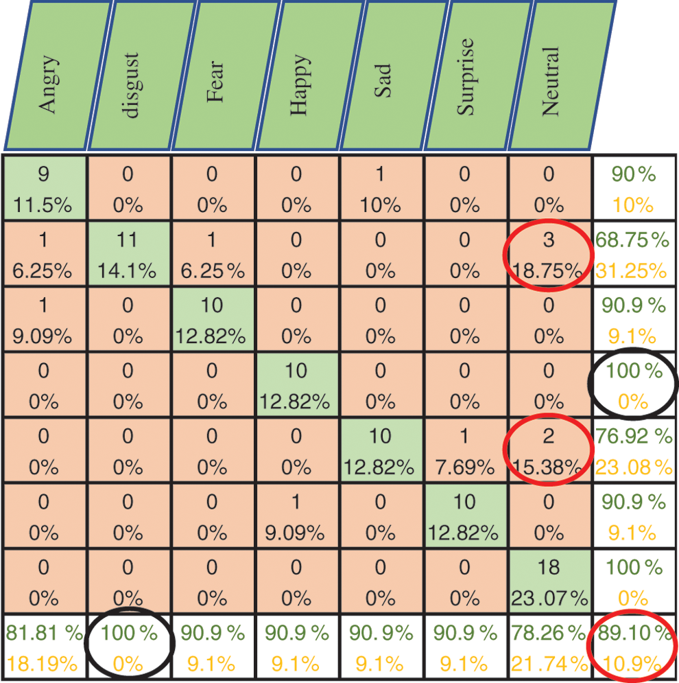
Figure 8: Exp1.1, SERS, FC-CSI, confusion matrix with SAVEE, without FS

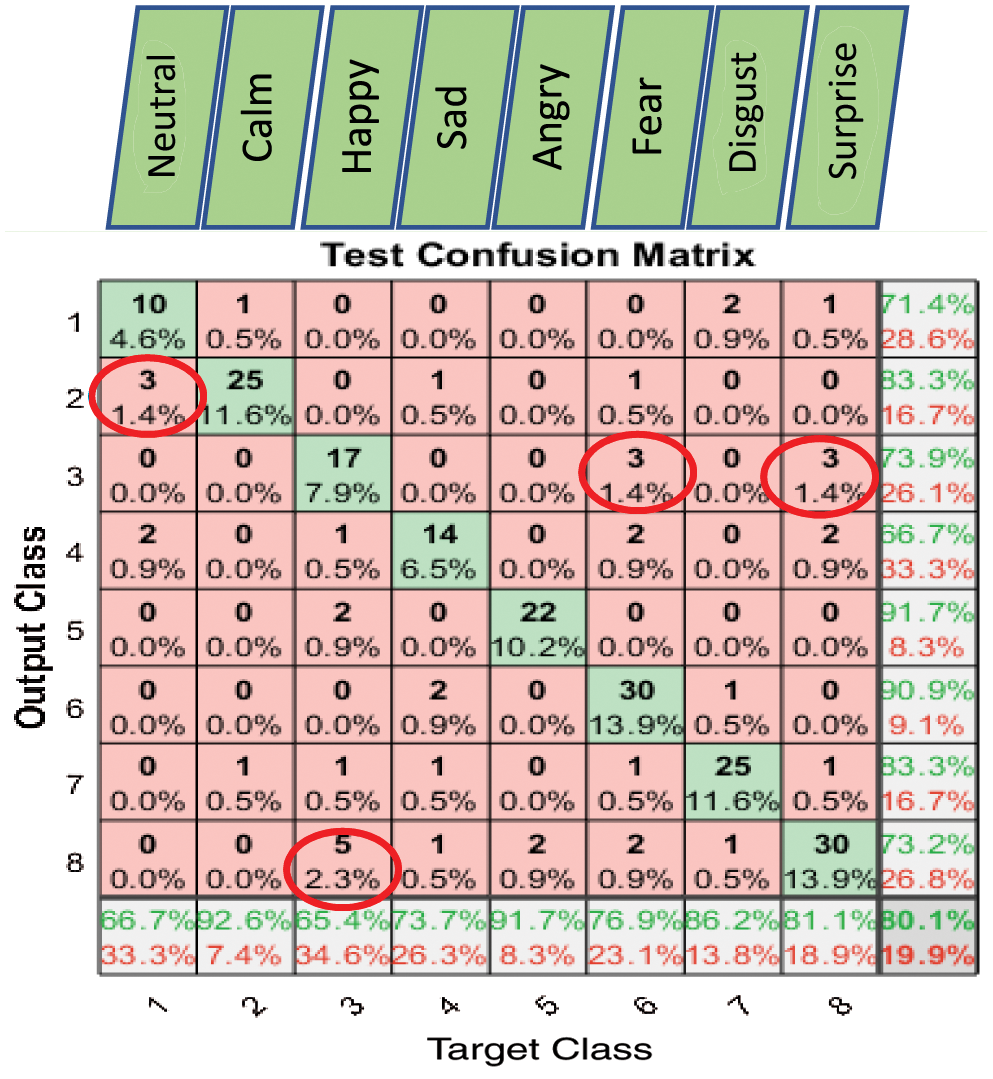
Figure 9: Exp1.1, SERS, SER-NN, confusion matrix with RAVDESS, without FS

3.1.2 SERS Influence on Dataset and Emotion

Fig. 12 shows the results of Exp1.1, the influence of the FC-CSI and SER-NN classification algorithms on the three datasets, and the emotions represented in those datasets.

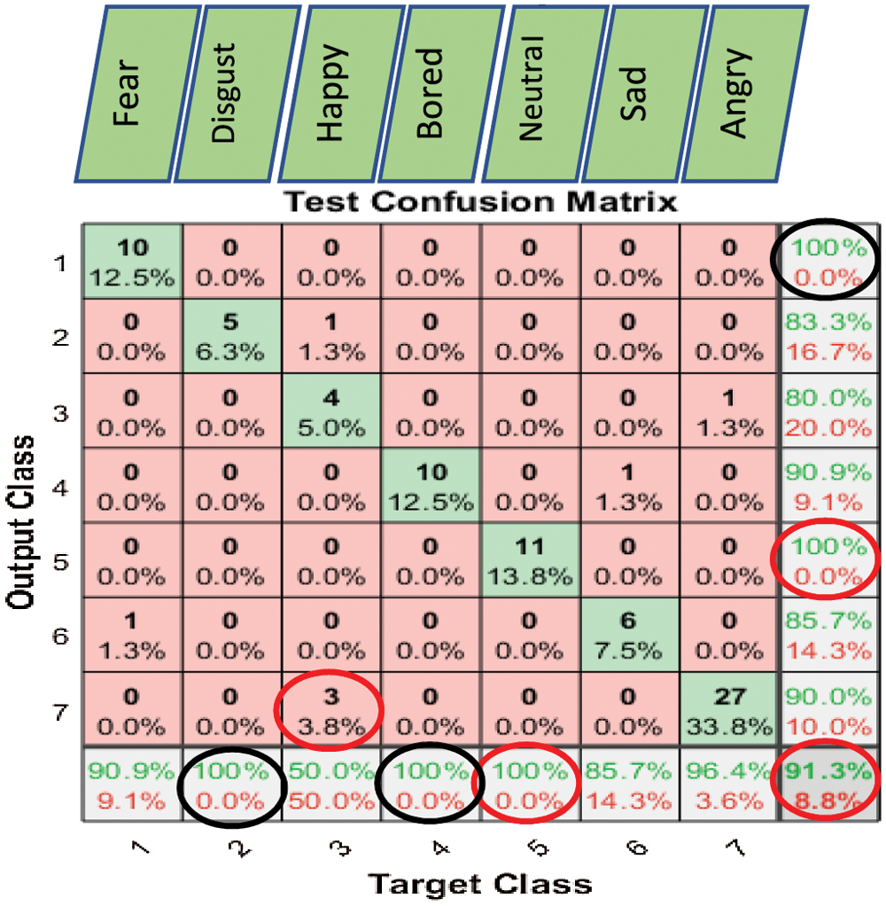
Figure 10: Exp1.1, SERS, SER-NN, confusion matrix with EMO-DB, without FS

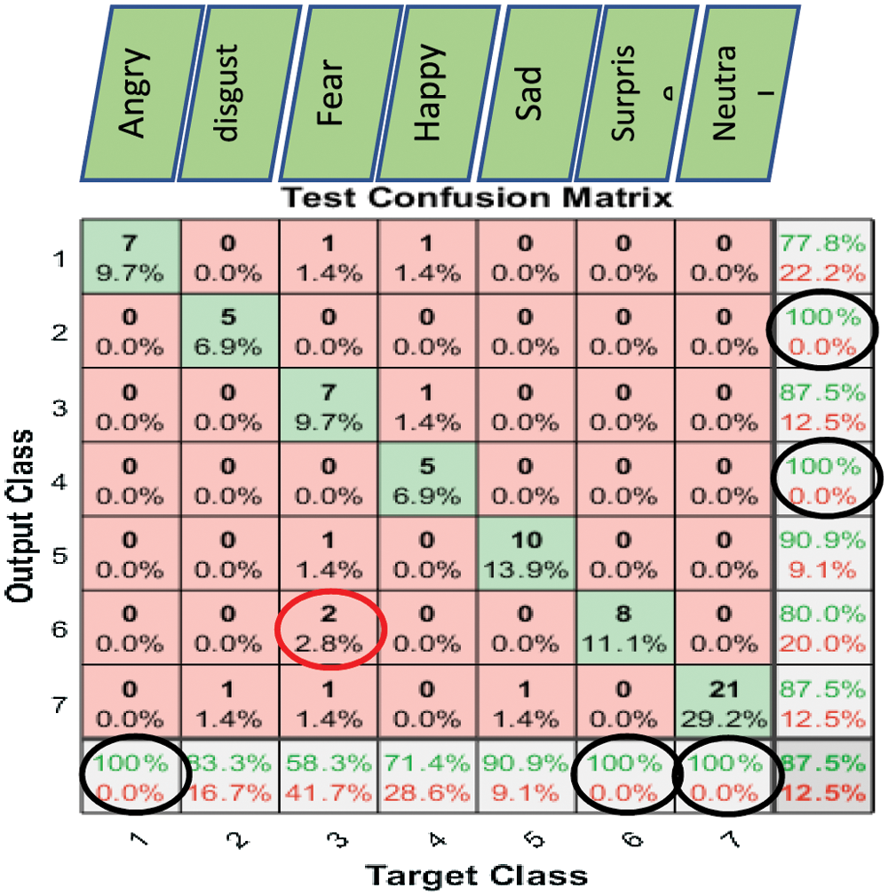
Figure 11: Exp1.1, SERS, SER-NN, confusion matrix with SAVEE, without FS

We observe the following:

•   FC-CSI showed lower performance for emotions with low amplitude, such as calm and bored;

•   FC-CSI showed average performance for emotions that contain many silent fragments, such as neutral;

•   FC-CSI failed to improve performance for the anger emotion on all three datasets;

•   The performance for all emotions of FC-CSI on RAVDESS did not appear similar to that of Emo-DB and SAVEE, except for the happy emotion, where FC-CSI performed better on all three datasets.

3.2 Experiment 1.2: SERS Performance Analysis After Deploying FS-TF Feature Selection Algorithm

Through Exp1.2, the classification performance of SERS was calculated by two different approaches, first utilizing the FC-CSI algorithm, and then SER-NN. Both approaches were implemented by deploying the FS-TF algorithm.

3.2.1 SERS Accuracy Performance

The column charts in Figs. 13 and 14 compare the performance of FC-CSI and SER-NN after applying FS-TF on the 2182 FE-MD features. FC-CSI suffered from feature selection because, with more features, the possibility of different shapes of CSI curves increased. Therefore, decreasing the number of features affected the performance of FC-CSI, but improved the performance of SER-NN.

Regardless of the best classification accuracy results gained from the NN, the proposed classification method accomplished the results shown in Tab. 3 using a smaller number of features, as shown in Tab. 4, which shows less complexity.

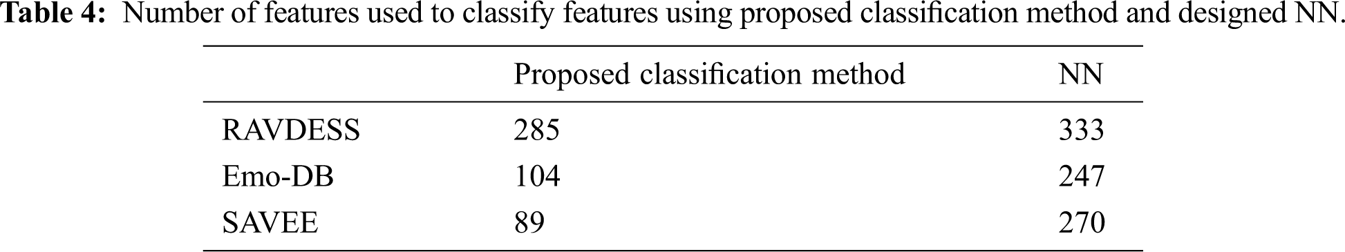
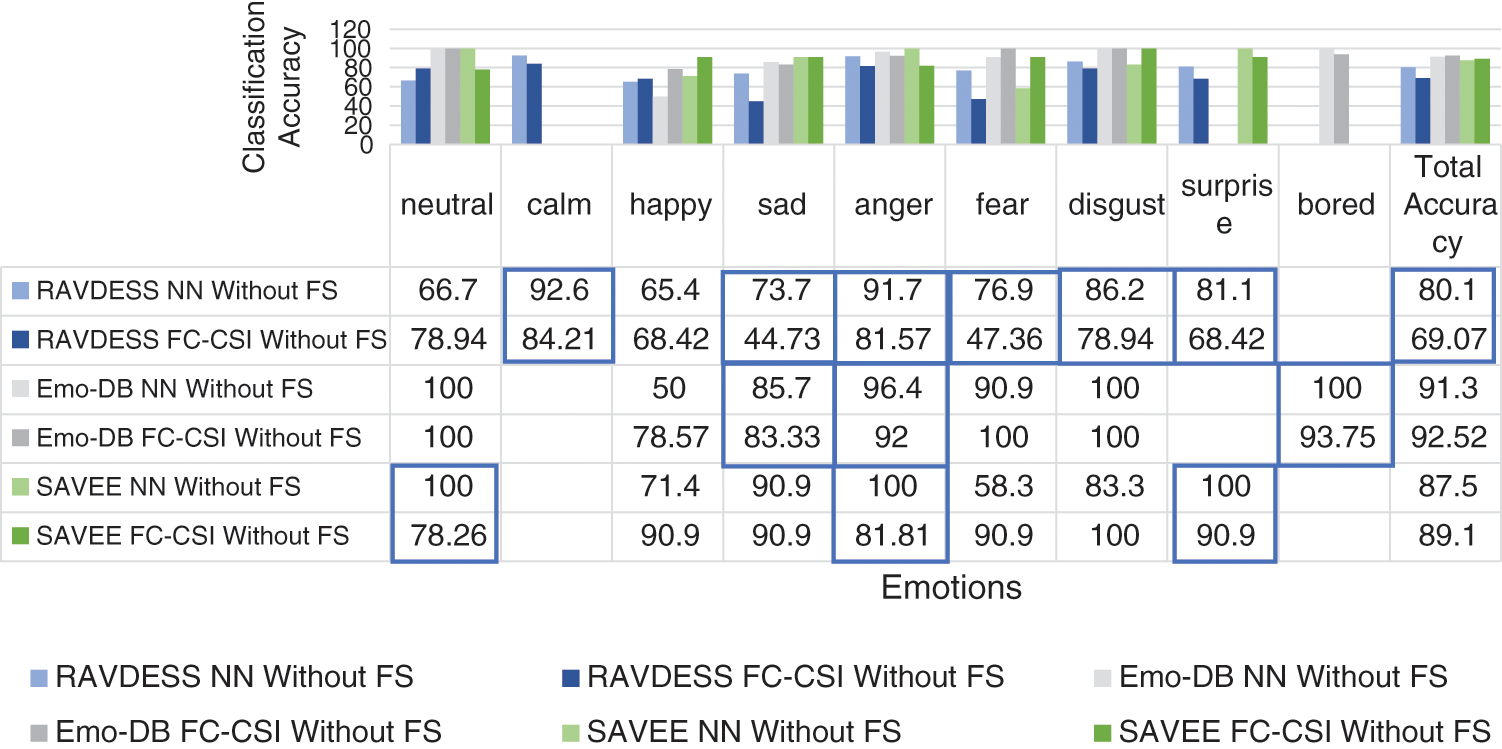
Figure 12: Exp1.1, SERS bar chart, result comparison between FC-CSI and SER-NN, without FS

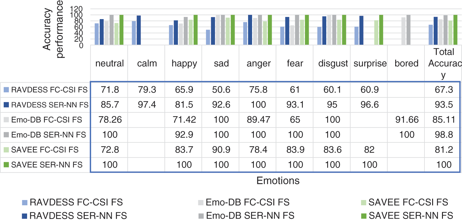
Figure 13: Exp1.2, SERS bar chart, results comparison between FC-CSI and SER-NN, with FS

3.2.2 SERS Influence on Dataset and Emotion

We compared the performance of FC-CSI before and after FS-TF to show how SERS suffered from the FS algorithm, and how it affected the emotions in each dataset (see Fig. 14). The results show that the neutral, calm, happy, anger, disgust, surprise, and bored emotions were quite affected by the FS algorithm, except for sad and fear, which means that FS generally affected the performance of FC-CSI on all three datasets.

3.2.3 General Clarification Aspects of FC-CSI Algorithm Performance

We clarify the results of FC-CSI. As discussed, the algorithm finds MCSI curves through the mean of 80% of the audio samples in the dataset, where each MCSI represents a different emotion. We find the Euclidean distance between the CSIs of each audio sample in the testing samples and classify each sample to the nearest MCSI. The MCSI curves that represent the emotions in RAVDESS, Emo-DB, and SAVEE are shown in Figs. 15–17, respectively.

It is obvious from looking at the curves in Figs. 15–17 that the MCSI curves related to Emo-DB and SAVEE are not similar. They intersect in some areas and are parallel in others, but as observed, each MCSI curve has a part that is not similar to any other MCSI curve in the same dataset, whereas the RAVDESS MCSI curves are parallel in many areas and intersect in others, which indicates the low performance of FC-CSI with RAVDESS.

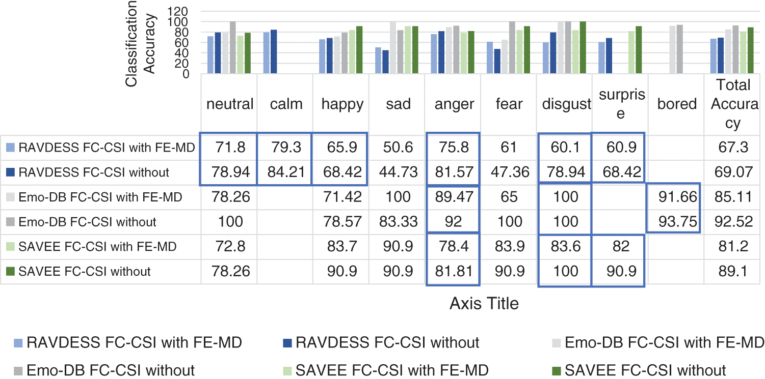
Figure 14: Exp1.5, SERS bar chart, results comparison study between FC-CSI before and after FS

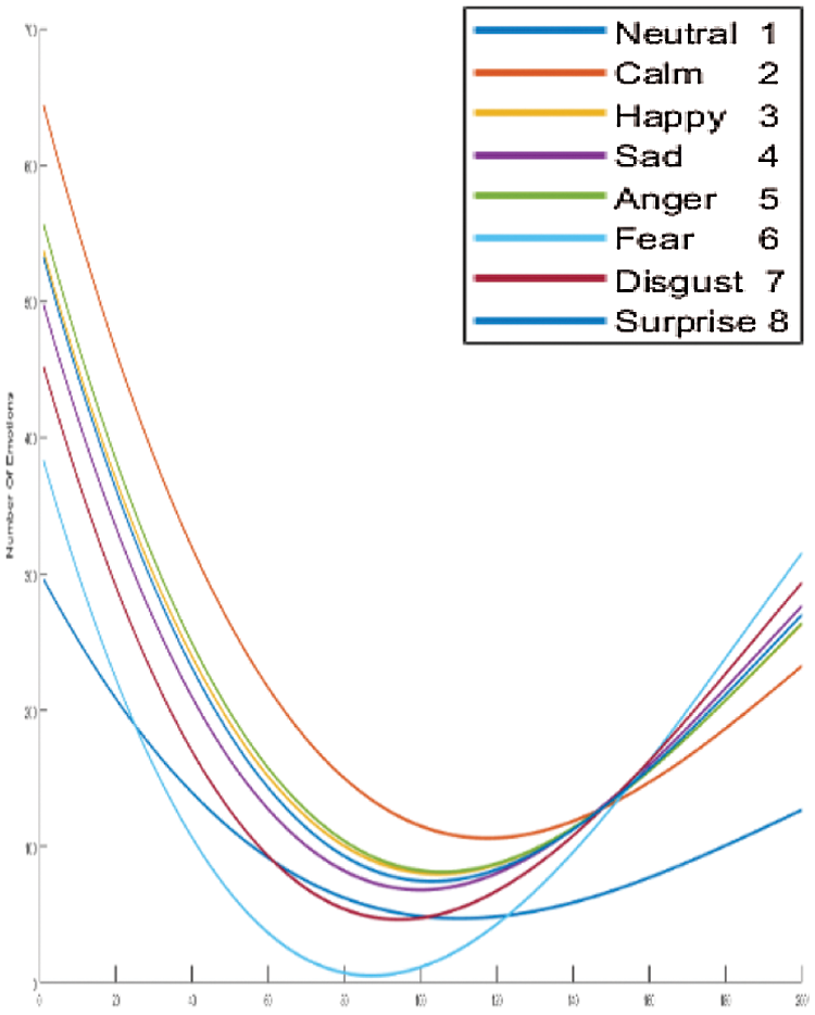
Figure 15: Exp1.1, SERS MCSI curves with RAVDESS, without FS

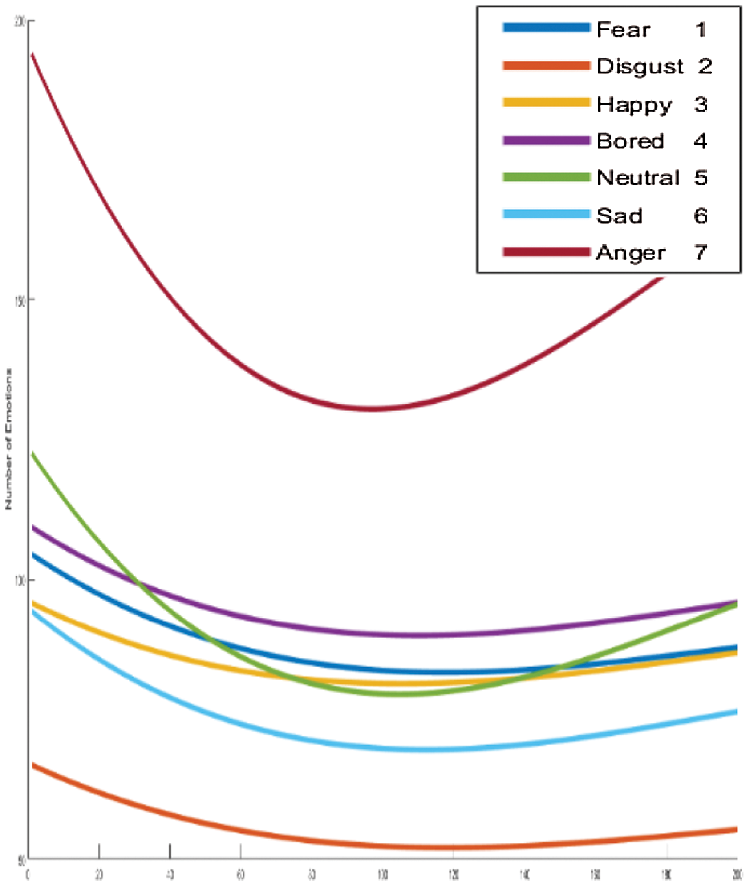
Figure 16: Exp1.1, SERS MCSI curves with EMO-DB, without FS

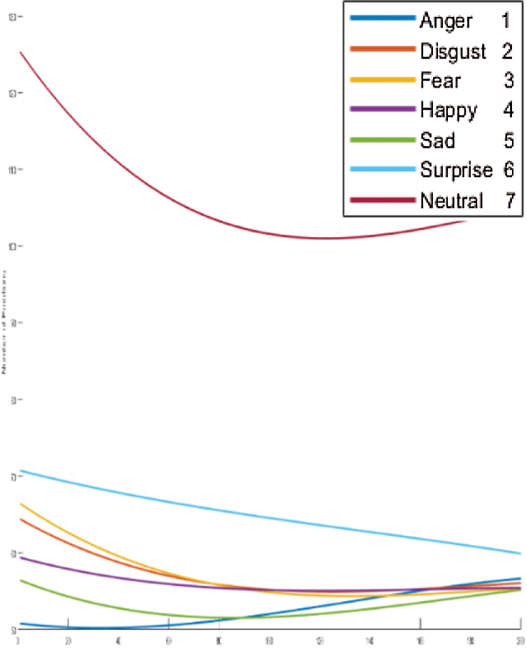
Figure 17: Exp1.1, SERS MCSI curves with SAVEE, without FS

4  Conclusions and Future Work

FC-CSI introduces a new research area in classification. No related work was found that deployed curves in classification, specifically the CSI. The most important conclusion is that CSI is a powerful data analysis tool. Splines correlate data efficiently and effectively, no matter how random the data may seem. Once the algorithm for spline generation is produced, interpolating data becomes easy. It was also noticed that statistical classification methods need less time than SER-NN methods, because SER-NN’s need time to learn and validate, whereas statistical methods require no learning. A set of speech signals representing a certain emotion shares a similar CSI behavior, which can be used in SER systems. Curve classification does not suffer from distinguishing conflicted emotions such as calm and neutral, or happy and anger, and they are gender-, speaker-, and language-independent. Possible future work based on this work is as follows. First, it would be more challenging to develop the proposed classification algorithm to deal with audio samples of unequal length. Second is to deploy a more complex distance measurement function, such as Fréchet distance. Third, we used CSI, but it is worth trying other types of curves, such as Bezier curves, with a higher dimension, such as three dimensions.

The proposed FC-CSI classification algorithm can also be applied to voice, speaker, and gender recognition, and can be used in classification systems such as image detection and object recognition. It can also be used to detect diseases and infections.

Acknowledgement: Thanks, and appreciation to everyone who contributed to this scientific research, especially the researchers cited in this paper.

Funding Statement: The author(s) received no specific funding for this study.

Conflicts of Interest: The authors declare that they have no conflicts of interest to report regarding the present study.

This work is licensed under a Creative Commons Attribution 4.0 International License, which permits unrestricted use, distribution, and reproduction in any medium, provided the original work is properly cited.