Intelligent Automation & Soft Computing DOI:10.32604/iasc.2022.019848
Article

Hysteresis Compensation of Dynamic Systems Using Neural Networks

Jun Oh Jang*

Department of Software Engineering, Uiduk University, Gyeongju City, 380004, Korea
*Corresponding Author: Jun Oh Jang. Email: jojang@uu.ac.kr
Received: 28 April 2021; Accepted: 11 June 2021

Abstract: A neural networks(NN) hysteresis compensator is proposed for dynamic systems. The NN compensator uses the back-stepping scheme for inverting the hysteresis nonlinearity in the feed-forward path. This scheme provides a general step for using NN to determine the dynamic pre-inversion of the reversible dynamic system. A tuning algorithm is proposed for the NN hysteresis compensator which yields a stable closed-loop system. Nonlinear stability proofs are provided to reveal that the tracking error is small. By increasing the gain we can reduce the stability radius to some extent. PI control without hysteresis compensation requires much higher gains to achieve similar performance. It is not easy to guarantee the stability of such highly nonlinear dynamical system if only a PI controller is used. Initializing the NN weights is simple. The initial weights of hidden layer are randomly selected and initial weights of output layer are set to zero. A PI loop with integerted an unity gain feedforward path keeps the system stable until the NN starts learning. Simulation results show its efficacy of the NN hysteresis compensator on a system. This work is applicable to xy table-like precision control system and also shows neural network stability proofs. Moreover, the NN hysteresis compensation can be further extended and applied to dead-zone, backlash, and other actuator nonlinear compensation.

Keywords: Hysteresis compensation; neural networks; dynamic inversion; velocity control

1  Introduction

Industrial dynamical control systems have generally the structure of a nonlinear system in front of some nonlinearity in the actuator, for example, dead-zone, backlash, and hysteresis, etc. Hysteresis phenomena caused by magnetism, stiction or gear with backlash generally exist in control system [1–3] and often severely reduce system performance such as giving rise to oscillations and/or undesirable inaccuracy, even leading to instability. Hysteresis characteristics are usually unknown and/or generally non-differentiable nonlinearities. Most results of adaptive control system are for differentiable nonlinear or linear systems, and are not applicable to control systems with non-differentiable nonlinearities. Developing an adaptive control scheme for systems with unknown hysteresis is a challenge of practical primary concern. The controlled plant may or may not have been known and the hysteresis is considered unknown. The goal is to achieve tracking and stabilization under influence of unknown hysteresis. In recent years, several rigorously guided adaptive schemes for compensation of actuator nonlinearities have been provided in detailed studies [4]. Backlash compensation with dynamic inversion is shown in [5,6], where NN is used to eliminate the inversion error. Adaptive control of plants with unknown hysteresis was developed using an adaptive inverse scheme [7]. In [8–10], NN compensation of gear backlash-like hysteresis in the position control mechanism was proposed.

In this paper, the author presents a NN hysteresis compensation design for a system. A rigorous design procedure with validation is provided to generate a PI tracking loop using an adaptive neural network system in a feed-forward loop for hysteresis compensation. The authors derive practical limits for tracking errors through tracking error dynamics analysis, and investigate the performance of NN hysteresis compensator in the system from computer simulations.

2  Neural Networks

NN has been used widely in feedback control systems [11–14]. Most applications are temporary, with no proven stability. The proof of stability that exists almost invariably relies on the property of a universal approximation to NN [15,16]. The three-layer NN in Fig. 1 is composed of an input, a hidden, and an output layer. There are L neurons in the hidden layer and m neurons in the output layer. Multilayer NN is a nonlinear function from input space Rn to output space Rm. The NN output y is a vector with m components determined by the equation as the n components of the input vector x.

yi=∑k=1L[wikσ(∑j=1nvkjxj+vk0)+wi0];i=1,2,…,m(1)

where σ(∙), the hyperbolic tangent functions, vkj the weight of the interconnection from the input layer to the hidden layer, and wik the weight of the interconnection from the hidden layer to the output layer. The threshold offsets are described as vk0, wi0.

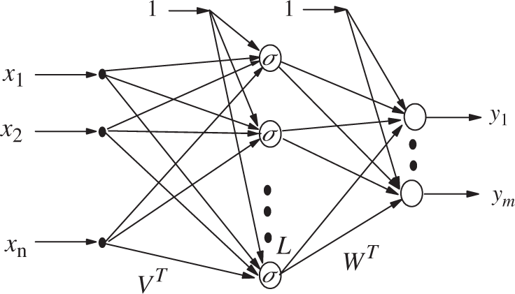
Figure 1: Three-layer neural networks

By gathering all the NN weights vkj, wik into matrices VT, WT, we can write the NN equation as vector as follows:

y=WTσ(VTx)(2)

The threshold is placed as the first column of the weight matrix WT, VT. In other words, the vector x and σ(∙) needs to be incremented by placing ‘1’ as their first element. That is , x = [1 x1 x2  · · ·  xn]T. To express (1) in this equation, there is sufficient generality σ(∙) to take as a diagonal function from RL to RL, which is σ(z) = diag{σ(zk)} for a vector z = [z1 z2  · · ·  zL]T ∈ RL.

For the convenience of notation, the matrix of all weights is defined as follows.

Z=[WV].(3)

According to many well-known results, a sufficiently smooth functiony¯can be randomly approximated in a compact set with appropriate weights, i.e., using a three-layer NN

y¯=WTσ(VTx)+ε(x).(4)

Here, it is the NN approximation error ε(x), and ||ε(x)|| ≤ εN on a compact set S [17,18]. The approximating weights V and W are ideal target weights, and are assumed to be bounded, such that ||V||F ≤ VM, ||W||F ≤ WM, or ||Z||F ≤ ZM.

3  Hysteresis Nonlinearity

In this section, the author presents a hysteresis model and a hysteresis inverse model. The implementation of hysteresis inverse is provided in the following sections to develop an NN hysteresis compensation scheme for unknown hysteresis systems. Hysteresis compensation is performed using dynamic inversion compensation, which uses NN for dynamic inversion compensation [19]. Other types of hysteresis models, including backlash and electronics, can be identified from references [1–3]. However, general history models will not be convenient because they are complex. Here, we will use a simplified hysteresis model with most hysteresis properties.

Fig. 2 shows a hysteresis model. The hysteresis properties H(∙) with input u(t) and output T(t): T(t) = H(u(t)) are described by the constants mt, ct, mb, cb, mr, cr, ml, cl and two half-lines:

T(t)=mtu(t)+ct,u(t)>u1=ct+mlclml−mt(5)

T(t)=mbu(t)+cb,u(t)<u2=cb+mrcrmr−mb(6)

and two line segments:

T(t)=mr(u(t)−cr),u2≤u(t)<u3=ct+mrcrmr−mt(7)

T(t)=ml(u(t)−cl),cb+mlclml−mb=u4<u(t)<u1(8)

where u1, u2, u3, u4 are the values of u(t) at the four opposite “conners” of the quadrilateral.

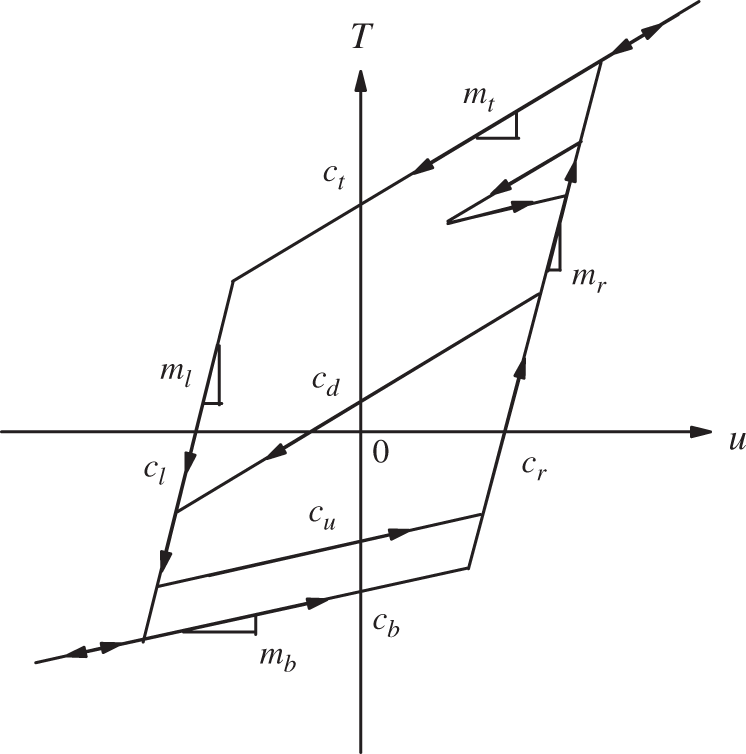
Figure 2: Hysteresis nonlinearity

Along the segments, the time derivatives of T(t), u(t) are of constant sign, namely, T˙(t)>0, u˙(t)>0 for T(t) = mr(u(t) − cr), and T˙(t)<0, u˙(t)<0 for T(t) = ml(u(t) − cl).

The hysteresis phenomena occur inside the loop formed by the half-lines (5) and (6) and the segments (7) and (8). Within the hysteresis loop, the relationship between T(t) and u(t) is

T(t)={mtu(t)+cd(t)foru˙(t)<0mbu(t)+cu(t)foru˙(t)>0(9)

where cd(t), cu(t)are partial constant function that depends on the point where u˙(t) changes the sign and the historical trajectories of (u(t), T(t)).

The motion of T(t) and u(t) inside the half-line (5) and (6) and the segments (7) and (8) and the hysteresis loop can be mathematically described as

T˙(t)={mtu˙(t)ifu(t)≥u3,orifu4<u(t)<u3,u˙(t)<0.T(t)≠ml(u(t)−cl)andT(t)≠mbu(t)+cb,orifu4<u(t)<u3,u˙(t)<0.T(t)=mbu(t)+cbandmt<mborifu4<u(t)<u3,u˙(t)>0.T(t)=mtu(t)+ctandmt<mbmbu˙(t)ifu(t)≤u4,orifu4<u(t)<u3,u˙(t)>0.T(t)≠mr(u(t)−cr)andT(t)≠mtu(t)+ct,orifu4<u(t)<u3,u˙(t)>0.T(t)=mtu(t)+ctandmt>mborifu4<u(t)<u3,u˙(t)<0.T(t)=mbu(t)+cbandmt>mbmru˙(t)ifu4<u(t)<u3,u˙(t)>0andT(t)=mr(u(t)−cr)mlu˙(t)ifu4<u(t)<u3,u˙(t)<0andT(t)=ml(u(t)−cl)0ifu˙(t)=0.(10)

Fig. 2 shows a hysteresis model and two typical minor loops. To cancel the hysteresis effect in the system, the pre-compensator must generate the reciprocal of the hysteresis nonlinearity. Fig. 3 shows the hysteresis inverse function. The dynamics of the NN hysteresis compensator is as follows

u˙(t)=Hinv(u,ud,u˙d)(11)

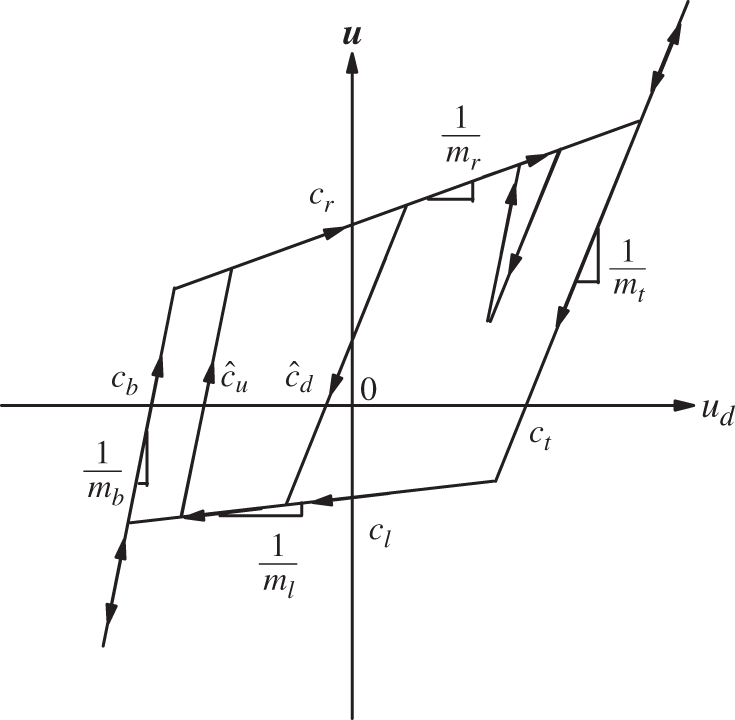
Figure 3: Hysteresis inverse

Also, Fig. 3 shows that hysteresis inverse properties can be decomposed into two functions. Fig. 4 shows the direct feed forward term and the further modified hysteresis inverse. This decomposition allows us to design compensator with better structure when NN is used in feed forward paths.

Figure 4: Hysteresis inverse decomposition (a) feed forward term (b) modified hysteresis inverse

4  NN Hysteresis Nonlinearity Compensation of Dynamic Systems

In this section, the author shows how to design an NN hysteresis compensator using back-stepping techniques [20]. It also shows how to weight or learn NN online, with small tracking errors and boundaries for all internal states (such as NN weights). Assume that actuator output can be measured. The system dynamics without vibration mode can be describes as follows.

Jθ¨+Bθ˙+Tf+Td=T(12)

where θ˙ is the motor velocity, J is the inertia, B is the viscous friction, Tf is the nonlinear friction components, Td is the bounded unknown disturbance, and T  is the control input. Supposed there is |Td| <  τM, with τM, a known positive constant. When a reference signal θ˙d is given, the tracking error is written by e=θ˙d−θ˙. The reference signal is restricted so that it is |θ˙d|<Θd with a known constant Θd. Using (12) we can differentiate tracking errors and write the plant dynamics in terms of tracking errors as follows

Je˙=−Be−T+f(x)+Td(13)

with the nonlinear plant function

f(x)=Jθ¨d+Bθ˙d+Tf(14)

The term x  includes all the time signals required for calculation f(∙), for example it can be defined as x≡[θ˙dθ¨d]T. Note that this function f(x) contains all potentially unknown functions without J, B as shown in (13) – this latter term is revoked from the stability proof. The following tracking controller provides a robust compensation scheme for unknown terms in f(x):

Tdes=Kfe+f^−v1(15)

with f^(x), an estimate for nonlinear terms f(x), v1(t) a robustifying term, and Kf > 0.

Fig. 5 illustrates the control structure implied by this scheme. The controller consists of a proportional and integral tracking loop with gains Kfe=KI∫e+Kpe and a hysteresis compensator that is enhanced by a hysteresis effect. We assume that non-linear function f(x) is unknown, but a fixed estimate f^(x) is known to satisfy function estimation error, f~(x)=f(x)−f^(x), |f~(x)|≤fM(x) for some known boundary functions fM(x).

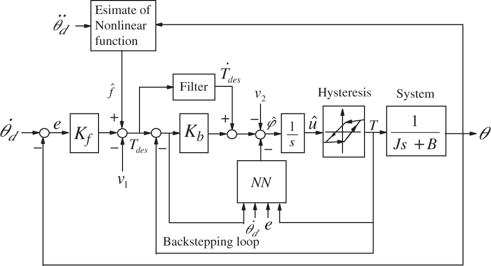
Figure 5: NN hysteresis compensation of systems

The following theorem is the first step in the backstepping design, which shows that the desired control law (15) keeps the tracking error small.

Theorem 1 : Under the system (12), use the tracking control law (15). Select the robustifying signal v1 as follows

v1(t)=−(fM(x)+τM)e|e|.(16)

the tracking error is then bounded and can be kept as desired by increasing the gains Kf.

Proof : Choose the Layapnov function candidate

L1=12Je2.(17)

Differentiating L1 and using the assumption |J˙|=0 and Eq. (13) yields

L˙1=e(−Be+f+Td−Tdes).(18)

Using the tracking control law (15) one has

L˙1=e(−Be+f+Td−Kfe−f^+v1)=−(Kf+B)e2+e(f~+Td+v1)(19)

L˙1=−(Kf+B)e2+e{f~+Td−(fM+τM)e|e|}.(20)

Eq. (20) can be bounded as

L˙1≤−(Kf+B)|e|2−|e|(fM+τM)+|e||f~+Td|.(21)

For as long as |e| ≠ 0, one can conclude that L˙1 is guaranteed negative.

Theorem 1 demonstrates a control law that guarantees stability in terms of tracking errors. If there is unknown hysteresis nonlinearity, the desired control signal and the actual value are different. According to the dynamic inversion concept, NN is used to compensate for the inversion error originally provided by Calise et al. [19], the author gives a rigorous analysis of closed-loop system stability. The actuator output provided in (15) is a desirable signal. To find the overall system error dynamics, define the error between the desired actuator output and the actual actuator output as follows:

T~=Tdes−T(22)

Differentiating one has

T~˙=T˙des−T˙=T˙des−H(T,u,u˙)(23)

which (13) and related (15) represent complete system error dynamics.

The dynamics of the hysteresis nonlinearity can be written as

T˙=ϕ(24)

ϕ=H(T,u,u˙)(25)

where ϕ(t) is pseudo-control input [19]. For known hysteresis, the ideal hysteresis inverse is given by

u˙=H−1(u,T,ϕ)(26)

Since hysteresis and thus its inverse are unknown, only the inverse of hysteresis can be approximated as

u^˙=H^−1(u^,T,ϕ^)(27)

We can now write the hysteresis dynamics as follows

T˙=H(T,u^,u^˙)=H^(T,u^,u^˙)+H~(T,u^,u^˙)=ϕ^+H~(T,u^,u^˙)(28)

where ϕ^=H^(T,u^,u^˙) and therefore its inverse u^˙=H^−1(T,u^,u^˙). The unknown function H~(T,u^,u^˙), that represent hysteresis inversion error are approximated using NN.

Introducing the NN approximation property, the hysteresis inversion error can be expressed as

H~(T,u^,u^˙)=WTσ(VTxnn)+ε.(29)

where the NN input vector is selected as xnn=[1eθ˙dT~T]T, and ε is the NN approximation error.

We define V^, W^ as estimates of the ideal NN weights provided by NN tuning algorithms. Define the weight estimation error as

V~=V−V^,W~=W−W^,Z~=Z−Z^,(30)

and the hidden layer output error for a given xnn as

σ~=σ−σ^=σ(VTxnn)−σ(V^Txnn).(31)

To design the stable closed-loop system with hysteresis compensation, nominal hysteresis inverse u^˙=ϕ^ and pseudo-control input ϕ^ are selected as

ϕ^=KbT~+T˙des−W^Tσ(V^Txnn)−v2(32)

where v2(t) is a robustifying term detailed later.

The closed loop system with NN hysteresis compensator is shown in Fig. 5. The proposed hysteresis compensation scheme follows the hysteresis inverse decomposition in Fig. 4. That is, the exact hysteresis inverse consists of a direct feed term and the error term in Fig. 4b estimated by NN.

The propod controller (32) allows to write the error dynamics (23) as

Taylor series expansions can be used to overcome the strong restriction of linearity in the tunable parameters. The weights V appear in nonlinear way. Applying the method developed in [15,16] yields the error dynamics

T~˙=−KbT~−W~T(σ^−σ^′V^Txnn)−W^Tσ^′V~Txnn+w+v2(34)

where the disturbance term is given by

w=−W~Tσ^′VTxnn−WTO(V~Txnn)2−ε.(35)

Here, O(V~Txnn)2represents a higher order terms in Taylor series expansion.

Assuming that the approximation property of the neural network are maintained, the norm of the disturbance term can be bounded as [15,16]

||w||≤VM||W~||F||xnn||+c1+c2||V~||F||xnn||+εN(36)

where c1 and c2 are positive constants. The NN input is bounded by

||xnn||≤c3+|e|+Θd+|T~|+||Z~||F(37)

Combination of the inequalities (36) and (37) one has

||w||≤(VM||W~||F+c2||V~||F)(c3+|e|+Θd+|T~|+||Z~||F)+c1+εN(38)

||w||≤C0+C1||Z~||F+C2||Z~||F|e|+C3||Z~||F|T~|+C4||Z~||F2,(39)

where Ci are computable positive constants.

The following theorem explains how to adjust the neural network weights so the tracking error e(t) and T~(t) achieve small values, whereas the NN weights V^, W^ are close to V, W. That is, the weight estimation errors (30) are bounded.

Theorem 2. Let the desired trjectories be restricted. Choose the control input as (27). Select the robustifying signal v2 as

v2=−KZ1(||Z^||F+ZM)(T~+|e|T~|T~|)−KZ2|e|T~|T~|−KZ3(||Z^||F+ZM)2T~|T~|(40)

where KZ1>max(C2,C3), KZ2>1, and KZ3>C4. Let the estimated NN weights be given by the NN tuning algorithm

V^˙=−QxnnT~W^σ^′−kQ|T~|V^,W^˙=−S(σ^−σ^′V^Txnn)T~−kS|T~|W^(41)

with any constant matrices S = ST  >  0, Q = QT  >  0, and k  >  0 small scalar deign parameter. The tracking error e(t), error T~(t) and NN weight estimates V^, W^ are then bounded by the limits given by Eqs. (57) and (58). Also, the error T~(t) can be made arbitrarily small by increasing the gain Kb.

Proof : Select the Lyapnov function candidate

L=L1+12T~2+12tr(W~S−1W~)+12tr(V~Q−1V~)(42)

which weights both errors e(t) and T~(t), and NN weights estimation errors. Taking derivative

L˙=L˙1+T~T~˙+tr(W~TS−1W~˙)+tr(V~TQ−1V~˙)(43)

and applying (13) and (34) one has

L˙=e(−Be−T+f+Td)+T~(−KbT~−W~T(σ^−σ^′V^Txnn)−W^Tσ^′V~Txnn+w+v2)+tr(W~TS−1W~˙)+tr(V~TQ−1V~˙)(44)

L˙=e(−Be+f+Td−Tdes)+eT~+T~(−KbT~−W~T(σ^−σ^′V^Txnn)−W^Tσ^′V~Txnn+w+v2)+tr(W~TS−1W~˙)+tr(V~TQ−1V~˙)(45)

L˙=e(−Be+f+Td−Tdes)+eT~+T~(−KbT~+w+v2)+tr[W~T(S−1W~˙−(σ^−σ^′V^Txnn)T~)]+tr[V~T(Q−1V~˙−xnnT~W^Tσ^′)].5pc.(46)

Using (15) and tuning rules yields

L˙=e(−Be+f~(x)+Td−Kfe+v1)+eT~+T~(−KbT~+w+v2)+k|T~|tr[W~T(W−W~)]+k|T~|tr[V~T(V−V~)](47)

Applying the same inequality as for (20), expression (47) can be bounded as

L˙≤−(Kf+B)|e|2−|e|(fM+τM)+|e||f~+Td|+k|T~|||Z||F(ZM−||Z~||F)−Kb|T~|2+T~w+eT~−T~KZ1(||Z^||F+ZM)(T~+|e|T~|T~|)−T~KZ2|e|T~|T~|−T~KZ3(||Z^||F+ZM)2T~|T~|.(48)

Intorducing (39) and applying some norm properties, one can has

L˙≤−(Kf+B)|e|2−|e|(fM+τM)+|e||f~+Td|+k|T~|||Z||F(ZM−||Z~||F)−Kb|T~|2+|T~||e|+C0|T~|+C1|T~|||Z~||F+C2|T~|||Z~||F|e|+C3||Z~||F|T~|2+C4|T~|||Z~||F2−KZ1|T~|2||Z~||F−KZ1|e||T~|||Z~||F−KZ2|T~||e|−KZ3|T~|||Z^||F2 ,(49)

L˙1≤−(Kf+B)|e|2+kZM|T~|||Z~||F−k|T~|||Z~||F2−Kb|T~|2+|T~||e|+C0|T~|+C1|T~|||Z~||F+C2|T~|||Z~||F|e|+C3||Z~||F|T~|2+C4|T~|||Z~||F2−KZ1|T~|2||Z~||F−KZ1|e||T~|||Z~||F−KZ2|T~||e|−KZ3|T~|||Z^||F2.(50)

Taking KZ2>1 yields

L˙≤−(Kf+B)|e|2+kZM|T~|||Z~||F−k|T~|||Z~||F2−Kb|T~|2+C0|T~|+C1|T~|||Z~||F+C2|T~|||Z~||F|e|+C3||Z~||F|T~|2+C4|T~|||Z~||F2−KZ1|T~|2||Z~||F−KZ1|e||T~|||Z~||F−KZ3|T~|||Z^||F2.(51)

Choosing KZ1>max(C2,C3) and KZ3>C4 one has

L˙≤−(Kf+B)|e|2+kZM|T~|||Z~||F−k|T~|||Z~||F2−Kb|T~|2+C0|T~|+C1|T~|||Z~||F(52)

L˙≤−(Kf+B)|e|2−|T~|[Kb|T~|+k||Z~||F2−(kZM+C1)||Z~||F−C0].(53)

Completing the square yields

L˙≤−(Kf+B)|e|2−|T~|[Kb|T~|+k{ ||Z~||F−(ZMk+C12k)} 2−k(ZMk+C12k)2−C0].(54)

Therefore, the L˙ is negative as long as

|T~|>k(ZMk+C12k)2+C0Kb,(55)

or

||Z~||F>ZMk+C12k+(ZMk+C12k)2+C0k.(56)

From the standard Layapnov theorem, the error, T~, decrease if the error is greater than the right side of (55). Eq. (57) gives a practical bound on the error

|T~|≤k(ZMk+C12k)2+C0Kb,(57)

Similarly, Eq. (56) gives

||Z~||F≤ZMk+C12k+(ZMk+C12k)2+C0k.(58)

Notice that by increasing the gain Kb we can reduce the stability radius to some extent. Also, note that PI control without hysteresis compensation requires much higher gains to achieve similar performance. Moreover, it is not easy to guarantee the stability of such highly nonlinear dynamical system if only a PI controller is used. NN hysteresis compensation demonstrates the stability of the system and can increase gain Kb to keep the tracking error arbitrary small. The NN weight errors are essentially constrained in terms of VM, WM. Due to the form of the feedforward compensator with integreted an unity feedforward path and a NN parallel path, initializing the NN weights is simple. The initial weights Vare randomly selected and initial weights W are set to zero. Then, a PI loop with integerted an unity gain feedforward path keeps the system stable until the NN starts learning.

5  Simulation Results

In this section, the author described the effective of a NN hysteresis compensator through computer simulations. One consider a plant with linear parts [21]:

G(s)=10.0143s+0.9785(59)

and the hysteresis characteristic H(mt, ct, mb, cb, mr, cr, ml, cl; ·) where mt = 1, mb = 0.5, mr = 4.0, ml = 5.5, ct = 0.5, cb = −0.5, cr = 0.3, cl = −0.3. The NN weight tuning parameters are chosen as S = 8I9, Q = 9I4, and k = 0.002, when IN is N × N identity matrix. The robustifying signal gains are KZ1=4, KZ2=2.5, and KZ3=6. The controller parameter Kp = 4, KI = 2, and Kb = 0.4. There are eight nodes in hidden layer in NN, i.e., L = 8. The input to hidden layer weights V is randomly initialized. Distributed uniformly between –1 and 1. The hidden to output layer weights W are initialized at 0. Because the weights W are initialized at zero, this weight initialization does not affect system stability, so initially there is no input to the system except for the PI loop. Filters that generates the signal T˙des is implemented as ss+100. Without the NN hysteresis compensation, the tracking performance of the closed-loop system is shown in Fig. 6.

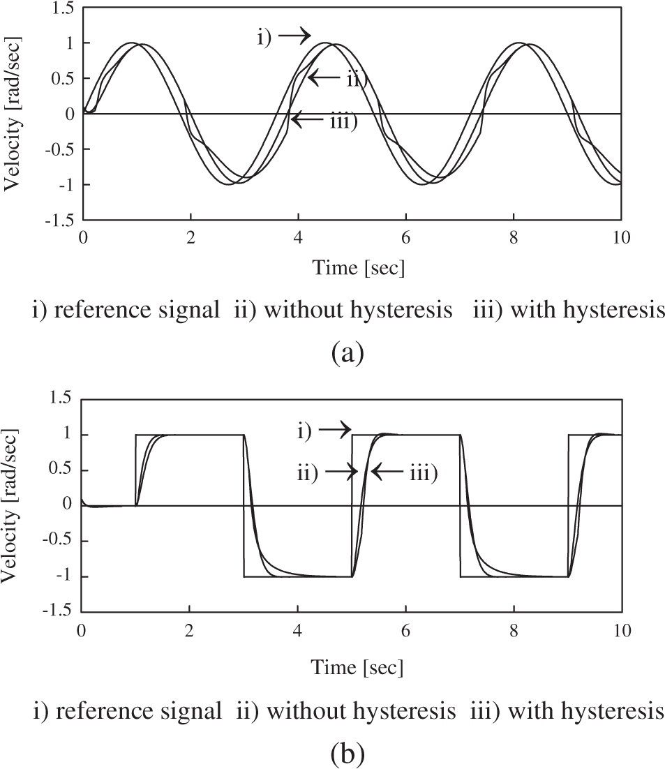
Figure 6: Velocity of a plant with/without hysteresis (a) sinusoidal reference signal (b) rectangular reference signal

Hysteresis causes a loss of information about the signal each time u(t) change direction, indicating that system performance is degraded. Applying the NN hysteresis compensator significantly reduces the tracking error. Fig. 7 shows the velocity of a plant when a NN compensator is included. Fig. 8 shows the control signal u(t) in both cases when NN is applied and when NN is not present. In the simulation it is clear that the proposed NN hysteresis compensation is an efficient method to compensate for hysteresis nonlinearities.

Figure 7: Velocity of a plant with/without hysteresis compensation (a) sinusoidal reference signal (b) rectangular reference signal

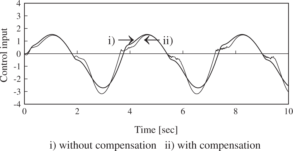
Figure 8: Control signal u(t) with/without NN hysteresis compensation

6  Conclusion

A new technique for the hysteresis compensation has been proposed for systems. The compensator scheme has a dynamic inversion structure, and the NN of the feed-forward path approximating the hysteresis inversion error and filter dynamics required for back-stepping design. We show how to adjust the NN weights so that the hysteresis inversion error is learned on line. Using nonlinear stability techniques, the boundaries for tracking error are derived from the tracking error dynamics. Through simulation, we show the significant improvement in system performance by NN hysteresis compensation scheme.

Acknowledgement: Author thank to anonymous reviewers for paper improvement.

Funding Statement: The author received no specific funding for this study.

Conflicts of Interest: The authors declare that they have no conflicts of interest to report regarding the present study.

This work is licensed under a Creative Commons Attribution 4.0 International License, which permits unrestricted use, distribution, and reproduction in any medium, provided the original work is properly cited.