DOI:10.32604/iasc.2022.016075
| Intelligent Automation & Soft Computing DOI:10.32604/iasc.2022.016075 | |
| Article |
A Time-Efficient and Exploratory Algorithm for the Rectangle Packing Problem
1Computer Engineering Department, Imam Khomeini International University, Qazvin, Iran
2Faculty of Science and Technology, University of the Faroe Islands, Faroe Islands
*Corresponding Author: Morteza Mohammadi Zanjireh. Email: Zanjireh@eng.ikiu.ac.ir
Received: 22 December 2020; Accepted: 29 April 2021
Abstract: Today, resource waste is considered as one of the most important challenges in different industries. In this regard, the Rectangle Packing Problem (RPP) can affect noticeably both time and design issues in businesses. In this study, the main objective is to create a set of non-overlapping rectangles so that they have specific dimensions within a rectangular plate with a specified width and an unlimited height. The ensued challenge is an NP-complete problem. NP-complete problem, any of a class of computational problems that still there are no efficient solution for them. Most substantial computer-science problems such as the traveling salesman problem, satisfiability problems (sometimes called propositional satisfiability problem and abbreviated SAT or B-SAT), and graph-covering problems are belong to this class. Essentially, it is complicated to spot the best arrangement with the highest rate of resource utilization by emphasizing the linear computation time. This study introduces a time-efficient and exploratory algorithm for the RPP, including the lowest front-line strategy and a Best-Fit algorithm. The obtained results confirmed that the proposed algorithm can lead to a good performance with simplicity and time efficiency. Our evaluation shows that the proposed model with utilization rate about 94.37% outperforms others with 87.75%, 50.54%, and 87.17% utilization rate, respectively. Consequently, the proposed method is capable to of achieving much better utilization rate in comparison with other mentioned algorithms in just 0.023 s running-time, which is much faster than others.
Keywords: Rectangle packing problem; best-fit algorithm; lowest front-line strategy
Decreasing wasting of resources affecting industries and businesses can be very advantageous [1–7]. The rectangle packing problem (RPP) is one of the most practical issues in the industrial sector. The RPP has many uses in various industries, including cutting leather, wood, metals, paper, glass, cloth, and paperboard [8–11], for designing and manufacturing cars, fighters, and ships [12–14], very-large-scale integration (VLSI) design [11,15–17], and even in similar issues like timing and replacement [18,19]. It also has uses in the assignment and timing of the radio frequency spectrum [18].
In the RPP, there exists a set of rectangles with specific dimensions, and the aim is to arrange these rectangles in a rectangular page with a fixed width and an unlimited height without overlapping, provided that the packing is orthogonal [20]. It means that the sides of the rectangles that are inserted into the rectangular page are parallel to the sides of the central page’s rectangle [16,21]. Also, the problem may not be guillotine-cut. That means that the replaced rectangles cannot be placed in several groups separated from the others by vertical or horizontal lines [8,17]. Rotation of the rectangles is acceptable, but the rotation angle could be only 90 degrees [22,23].
In addition to waste reduction, increasing the utilization rate is one of the fundamental challenges in the industry. The utilization rate equals the sum of the area of the input rectangles (
In this equation, width represents width of the main page, and height represents height of the main page, (wi) and (hi) are the width and height of the replaced rectangles, respectively, and m is the number of these rectangles [22].
In the past decades, various related algorithms have been presented due to its crucial role and importance in the widespread applications. Despite a wide range of the RPP applications, the efficient implementation is still a complicated task. The most fundamental challenge is that we should solve an NP-complete set problem [20,24,26–29]. Therefore, with an increase in the problem scale, achieving a practical solution with an appropriate run time could be difficult or even impossible.
The rest of this article is organized as follows. In the second section, the related works about the rectangle packing context were discussed. In the third section, the methodology with the proposed algorithm was presented in full detail. In the fourth section, achieved results were presented, and ultimately the fifth section dealt with the conclusion.
To solve the RPP, one of the most favorite algorithms that has attracted many researchers is the Best-Fit algorithm. It is a multi-layered algorithm in which the layers are created gradually as the rectangles are inserted. The rectangle places into the higher level, if it cannot be placed in a layer. In conclusion, the rectangle will always be located in a layer that has less waste after insertion [8].
Hu et al. [11] have presented an algorithm based on Best-Fit and BL algorithms. Their algorithm has all of the properties of the two mentioned algorithms. This algorithm categorizes the rectangles first and then places the created categories one by one. This method is suitable for rectangles with different sizes but with some restrictions to the number of input rectangles. The time complexity of this algorithm is O(mMlogM), in which m and M could be equal to the number of input rectangles.
Liu et al. [22] presented a solution for the RPP by combining the lowest front-line algorithm with the genetic optimization algorithm. Arrangement of the rectangles from the lowest point possible to the highest point is a prominent feature of this algorithm that reduces space waste. It also utilizes a smart function to cross local optimum modes. The long-running time of this algorithm for identifying and improving various modes is its fundamental challenge.
Huang et al. [30] presented an algorithm based on two basic algorithms, including the Best-Fit algorithm and particle swarm optimization (PSO) algorithm. They compared their method with the presented classical methods and achieved more efficient results. However, the fundamental challenge of their approach is the long-running time of the algorithm.
Chazelle [31] introduced an algorithm called Bottom Left Fill (BLF). The number of possible modes for inserting a rectangle was decreased in the BLF algorithm. While in the BL algorithm, it is impossible to use the leftover spaces from placing the rectangles, in the BLF algorithm, the rectangle is placed at the lowest point possible. The BLF algorithm uses unused spaces. The time complexity of this algorithm is O(n2), where n is the number of inputs. This means that this algorithm is not scalable well.
Liu et al. [32] developed an algorithm for the RPP based on two algorithms, including the BL algorithm and the genetic algorithm (GA). They improved the initial BL algorithm because it does not identify some of the modes. As the mode in which the rectangles are alternately big and small, the big rectangles have ascending sizes, and the small ones have descending scales. The decisive point of this algorithm is the use of an intelligent crowd function for the GA (genetic algorithm). The running order of this algorithm is O(n2).
In this section, at first, two algorithms including the Best-Fit decreasing height algorithm and the lowest front-line strategy are introduced. Then, the researchers present the proposed model in this research in its details.
3.1 The Lowest Front-Line Strategy
An acceptable paper size is US Letter (
The lowest front-line strategy is designed based on the BL algorithm and is defined as follows [22]:
• The first step: The algorithm starts with the initial quantification of the front line. In the beginning, the front lines set contained only one line, and that is the horizontal line at the bottom of the page.
• The second step: Locating the rectangle in a place using the lowest front-line strategy. pi is the position where the i − th rectangle is placed. First, we select and check one line of the front line set to see whether the width of the rectangle that is going to place is equal to or smaller than the width of the selected line. If the conditions are true, that rectangle will be placed at the top left of the page. If the conditions are not true, the height of the lowest line is increased until it reaches the second lowest front line, and the conditions will be rechecked. This process repeats until one line of the front line set gets selected. In this step, if several lines exist with the lowest heights, the selection will be based on the X-axis. If height is increased from a lower line to a higher line, they will be merged.
• The third step: In this step, the front line will be updated. Some of the old lines will be converted to new lines, and new lines will be added to the front line set. As the points mentioned in the second step, the adjacent lines with equal height must be merged to form a single line.
• The fourth step: If all rectangles are placed, the algorithm ends, otherwise a new rectangle will be selected, and the process will continue to the second step.
Fig. 1 demonstrates an example of the lowest front-line strategy. P1 will be selected for {A1A5}, and after that, the front line will be {E1E2, A2A5}. In the same way, p2 will be selected for {A2A5}, and after the placement, the front line will be {E1E2, B1B3, A3A5}. Similarly, after placing the p3 rectangle in {A3A5}, the front line will be {E1E2, B1B3, C1C2, A4A5}. In this point, the lowest line is {A4A5}, and it does not have enough space to place P4. So, the height of {A4A5} was increased until it reaches {B1B3}, the second-lowest front line. Finally, the {B1B3} line will be selected to place the P4 rectangle, and the front line is {E1E2, D1D2, B2B3, c1c2, B4B5} at the end [22].
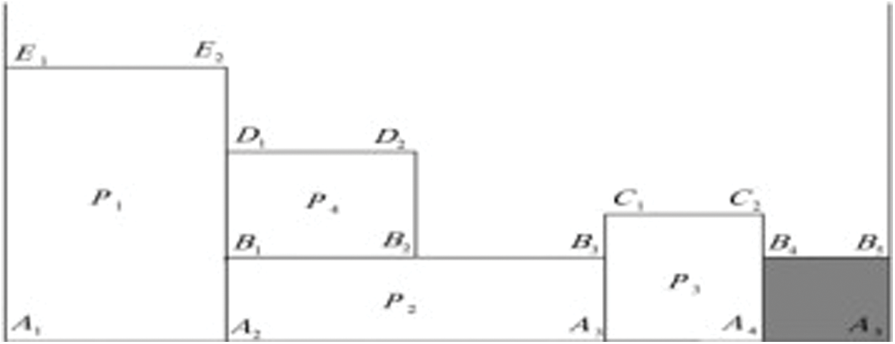
Figure 1: The lowest front-line strategy
The lowest front-line strategy does not sort the input rectangles before placing them. Actually, this is a challenge for this algorithm. It increases page height and decreases the utilization rate. This algorithm always tries to find the lowest and the leftmost point possible to place the rectangles. The way the height increases in this algorithm is its positive point.
3.2 The Best-Fit Decreasing Height Method
In the Best-Fit decreasing height algorithm, the rectangles are first sorted in decreasing order. Then, the biggest rectangle will be placed at the bottom-left corner, and the first layer will be created. To place the next rectangles, if the rectangles could not be placed in the created spaces of the created layer, we create a layer above the highest layer and place the rectangle in it. If there are several layers with enough space to place the rectangles, a layer will be selected with less waste after the rectangle placement [33,34]. The time complexity of this algorithm is O(nlogn) [35].
The Best-Fit decreasing height algorithm is layered well, and it is suitable for non-guillotine cut issues. Finding the best position with the lowest waste is waste is a noticeable advantage of this algorithm. Also, due to sorting the inputs, this algorithm has a better utilization rate compared to the Best-Fit algorithm without sorting. In this algorithm, we cannot place a rectangle between two layers, and this causes wasting. Therefore, we can place the rectangle between the layers in the proposed algorithm.
This study presents an algorithm with the properties of both Best-Fit decreasing height algorithm and the lowest front-line strategy. This algorithm, similar to the Best-Fit method, always tries to find the best position for the rectangle. However, this algorithm aims to decrease the total height by increasing the height of the layers, inspired by the lowest front-line strategy.
The steps of the proposed algorithm are as follows:
The first step: At first, the algorithm starts with initial quantification. The height of this page is zero initially, and its final value is specified at the end of the algorithm. In this algorithm, there exist a set of lines called the front line for saving empty spaces. In the beginning, the front line is the bottom borderline of the page. The information of the input rectangles such as width, height, and the number of each one will be received at this stage of the algorithm.
In this algorithm, an array was used to reserve empty spaces. The first row of this front-line array is the starting point of the line, the second row of the front-line shows the endpoint of the line, the third row of the front-line array represents the distance of this line from the lowest front line, which is the bottom borderline of the page, and the fourth row of the front-line array shows the height of the next front-line after this line. With these four points, we can imagine a rectangle. If the value of the fifth row of the front-line array is 1, it means that this line is not occupied, and when a rectangle is placed, this value will become −1. The fifth row of the array is added to adhere to the not-overlapping assumption. When placing rectangles into a line using the fifth row of the front-line array, it will be checked whether it is full or empty.
The second step: In this step of the algorithm, the rectangles with more height than width will be rotated 90 degrees. It means that the height and the width will be replaced.
The third step: In this step, the rectangles will be sorted in decreasing height size order.
The fourth step: A rectangle will be selected from the beginning of the inputs list, and then, we search among the front-lines set for a place with enough space for the rectangle. Then, among the selected lines, we choose a line that has less waste. At this point, there are three modes:
• If a line is found among the front-lines set with sufficient width and height for placing the rectangle, we select it; and if there are several lines for placing, we choose the one that wastes less space.
• If we cannot find a line with the required height and width, we start searching among the longest front-lines for a line that has the required width for placing the rectangle. Also, if there are several lines, we choose the one that has less width and increases the height of the page lesser.
• If we cannot find a position to place the rectangle in the two predicted modes mentioned above; and if we did not find any line that has enough space for placing the rectangle, then we create a new layer above the longest front-line and place the rectangle in the bottom-left of the created layer and increase the height of the page.
The fifth step: In this step, we update the front-line and empty spaces, and convert some of the old lines into new lines and also add new lines. In addition, we must identify all of the empty spaces. Then, we try to identify all of the empty houses that have common borders. In order to make the most of the wasted space available, if one or more than two houses have common borders, it must be merged with the house that creates larger free space after merging compared to other houses. This step plays an essential role in reducing waste.
The sixth step: In this step, we check the ending of the algorithm. If there is not a rectangle in the input list to place, the algorithm ends. Otherwise, we go to the beginning of the fifth step and continue the algorithm again. In the end, we calculate the utilization rate of the algorithm. Fig. 2 shows the flowchart of the algorithm process.
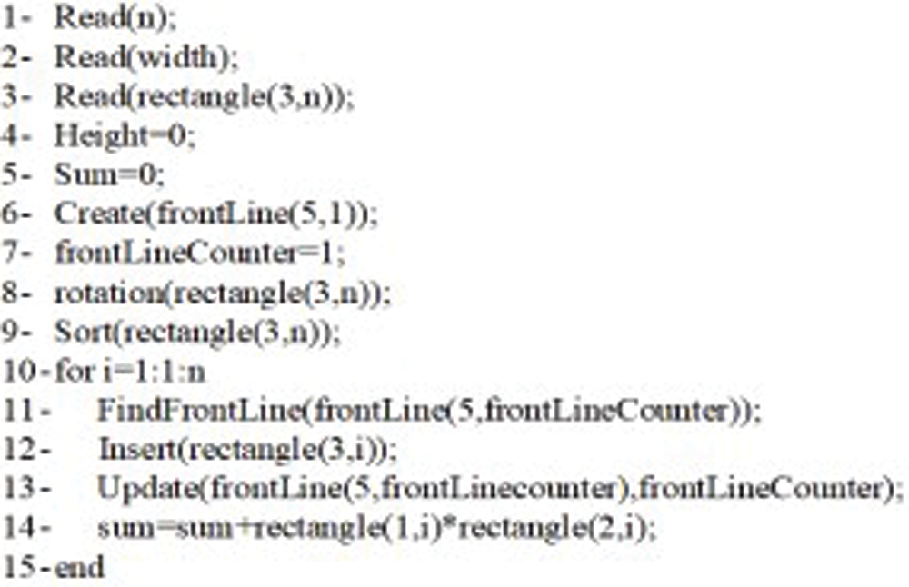
Figure 2: The semi-code of the proposed algorithm
In this study, the MATLAB programming language was used in a PC with Intel(R) Core(TM) i7 and 12 GB internal storage. The data was deployed using the Liu algorithm [22] for the evaluation of the algorithms. Tab. 1 shows these data, and also, the width of the rectangle page is 400 units. Then, the achieved results of the proposed algorithm were compared with the Liu study [22], Best-Fit, and front-line.
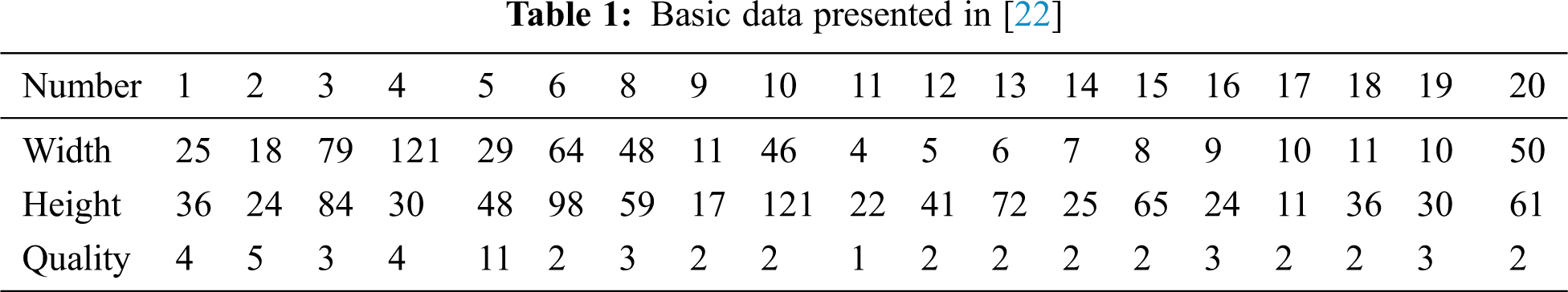
Tab. 2 shows the results of all mentioned algorithms. It indicates that the proposed algorithm has the best performance about 94.37% compared to 87.75%, 50.54%, and 87.17% for other algorithms. Besides, our method reached the utilization rate of 94.37% in just 0.023 s, well below others. Whereas the method presented in [22] reached the utilization rate average of 85.51% after 300 times repeating the algorithm and 26.3 s, and at best, it has reached the rate of 87.75%.
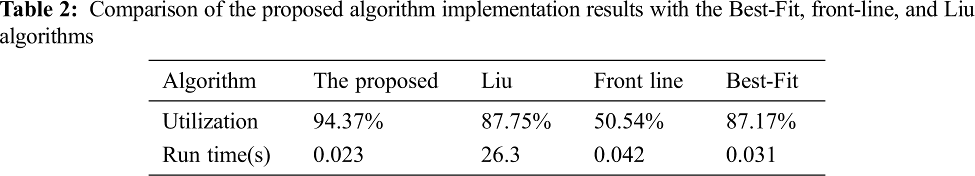
Fig. 3 plots the utilization rate of the three Best-Fit decreasing height, the lowest front-line strategy, and the proposed algorithms. In this figure, the utilization rate percentage of every algorithm has been drawn after placing each rectangle. The horizontal axis represents the number of placed rectangles, and the vertical axis represents the utilization rate percentage.
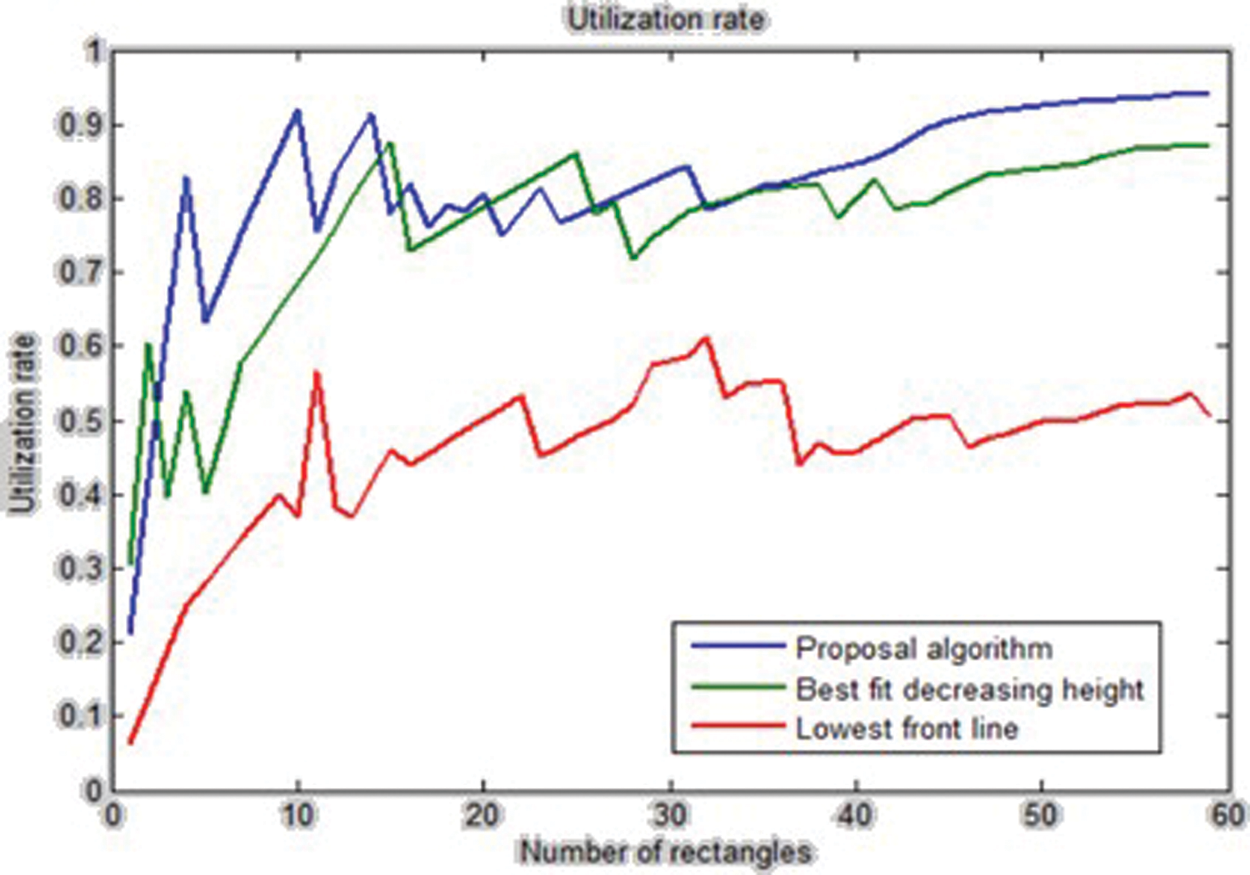
Figure 3: The utilization rate of the three Best-Fit decreasing height, the lowest front-line strategy, and the proposed algorithms
Fig. 4 shows the run time vs. number of rectangles of the three algorithms, including Best-Fit decreasing height, the lowest front-line strategy, and the proposed algorithm. In this figure, the best running time belongs to the proposed algorithm.
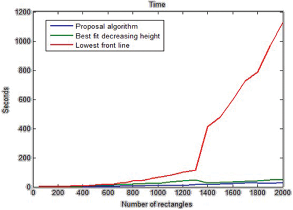
Figure 4: The running time of the Best-Fit decreasing height algorithm, the lowest front-line strategy, and the proposed algorithm
4.1 The Effect of the Sorting and Rotation on the Utilization Rate
In this section, we analyze the effects of the sorting and rotation on the utilization rate. Sorting the input rectangles has a significant impact on the utilization rate. We sorted the input rectangles in descending order of height, width, and area of the rectangles, and then we ran the algorithm. The results of running the algorithm show that sorting in descending order of height has better results. Tab. 3 shows the results of this comparison, and Fig. 5 shows the utilization rate for various sorting modes.
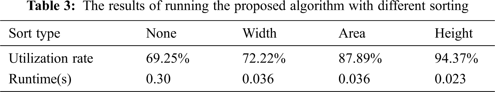
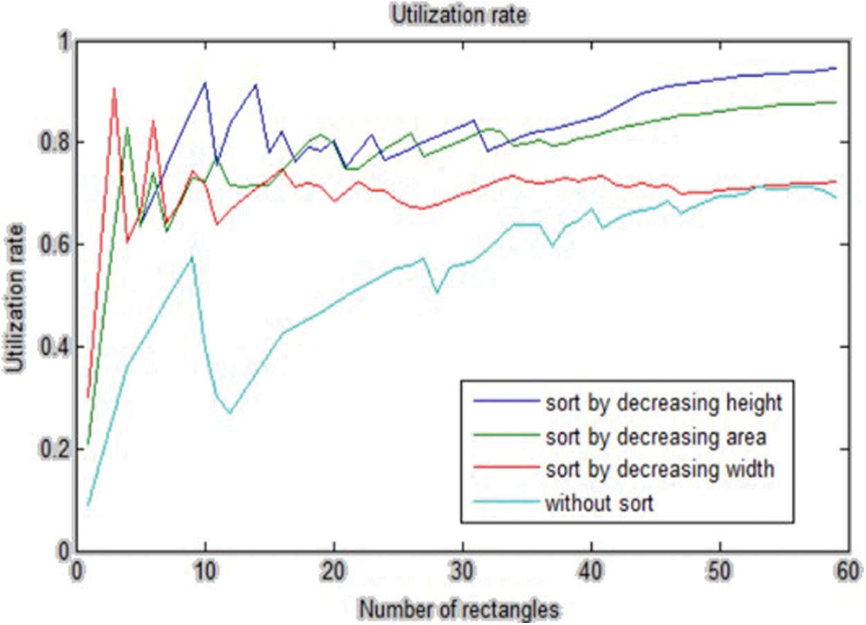
Figure 5: The utilization rate of the proposed algorithm with different sorting
The rotation step was removed to run the algorithm again. Then, the new results were compared with the algorithm while considering the rotation. The results showed that the rotation has a positive effect on the utilization rate. Tab. 4 shows the results of this experiment. Fig. 6 draws a comparison between running the algorithm with and without the rotation.
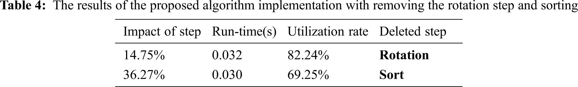
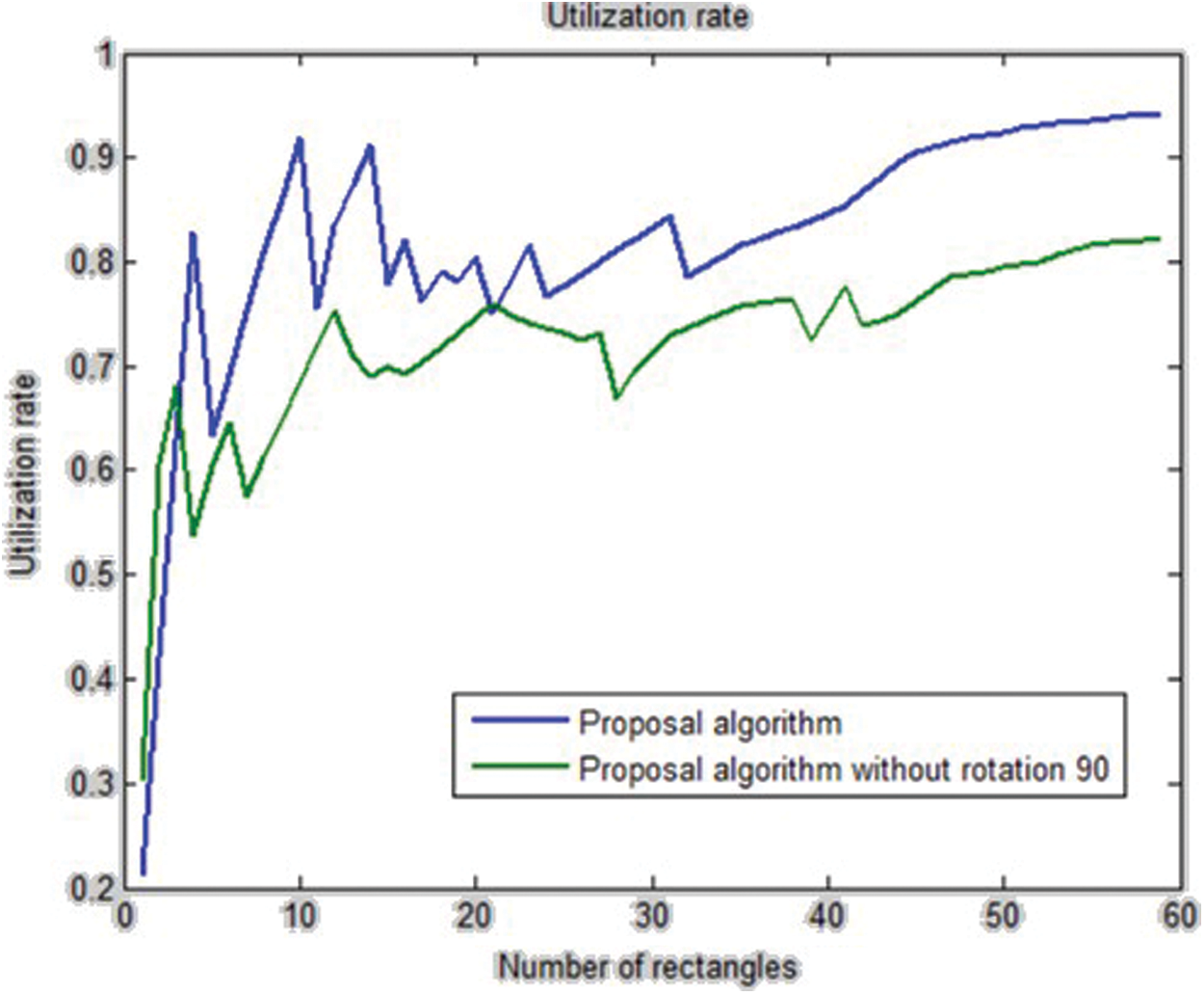
Figure 6: The utilization rate of the proposed algorithm with & without the rotation step
4.2 Comparing the Algorithm with Random Data
Comparing the algorithm with low-volume data and also, in some cases, comparing the algorithm with high-similarity data, is one of the challenges of the presented algorithms. Practically, there are various data with different sizes in the industry. Therefore, in this section, the proposed algorithm, the lowest front-line strategy, and the Best-Fit algorithm were analyzed by producing random data. The obtained results show that the utilization rate of the proposed algorithm is better than the other two algorithms. In addition, it has a shorter running time. Tab. 5 shows the utilization rate and the running time of these algorithms. Fig. 7 indicates the utilization rate of the Best-Fit, front-line, and proposed algorithms with random data. Also, Fig. 8 shows the running time of these three algorithms.
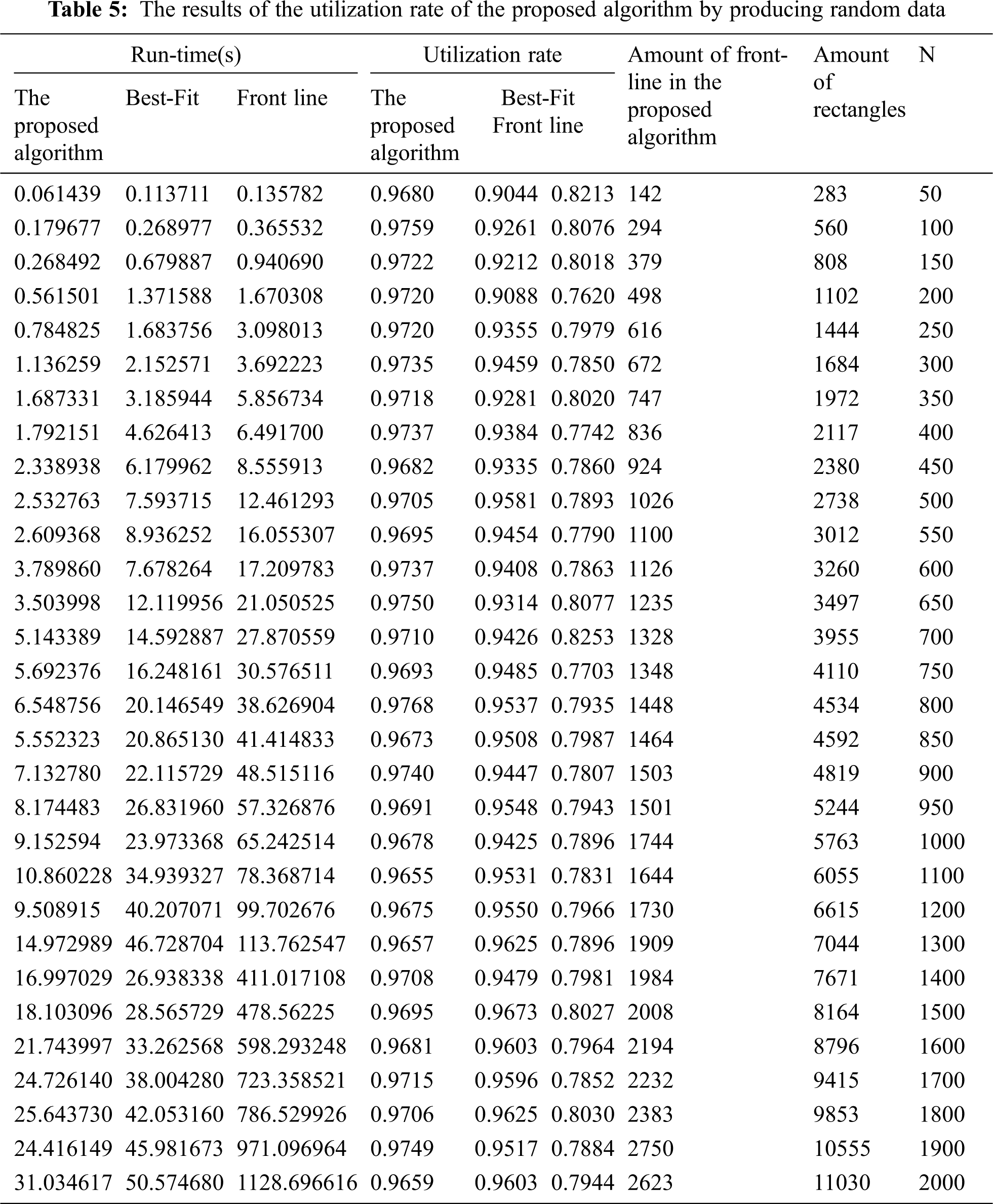
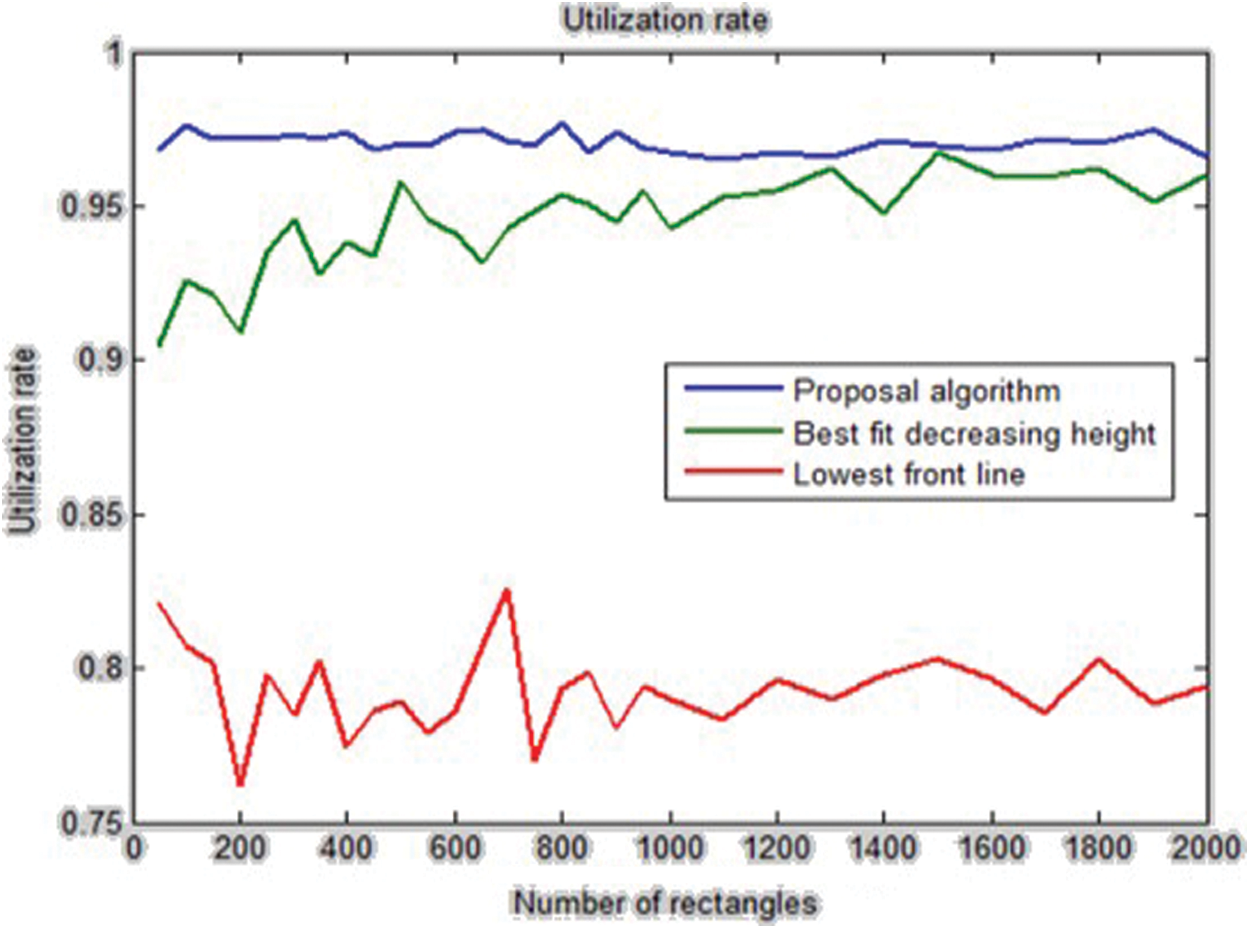
Figure 7: The utilization rate of the Best-Fit, front-line, and proposed algorithms with random data

Figure 8: The running time of the Best-Fit, the front-line, and the proposed algorithms with random data
The proposed method has the polynomial-time complexity. As a result, it needs maximum O(m) time for searching between m front-lines and finding the proper line to place the rectangle. This task must be done for all of the rectangles, and the total number of rectangles is n. Therefore, the time complexity of this algorithm is generally linear in time order and equals O(nm). The results of the implementation indicate that the value of m is always less than n. It means that at the end, the total number of the front-lines is always less than the total number of the rectangles. In Tab. 5, the total number of rectangles column is n, the total number of front-lines column is m, and m is always less than n. Fig. 9 demonstrates how the number of front-lines increases per number of input data.
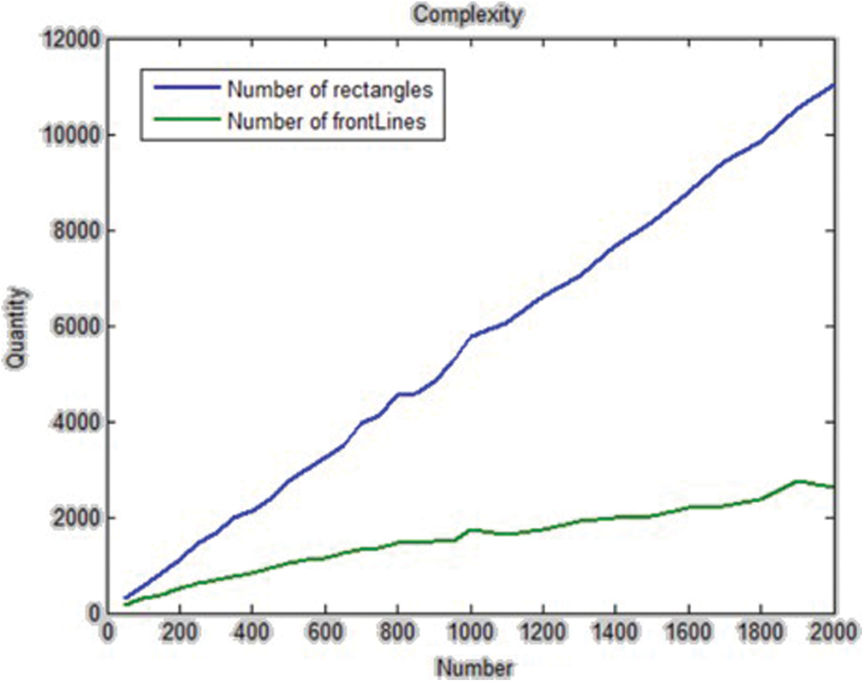
Figure 9: The comparison between the number of rectangles and the number of front-lines
In this study, an efficient algorithm was presented for the Rectangle Packing Problem (RPP). RPP struggles to insert a set of non-overlapped rectangles (with specific features) in a rectangular space (with a constant width and an unlimited height), providing that the packing is orthogonal. To this end, we have implemented the proposed algorithm along with the Best-Fit decreasing height and the lowest front-line strategy. Our evaluation shows that the proposed model with utilization rate about 94.37% outperforms others with 87.75%, 50.54%, and 87.17% utilization rate, respectively. Consequently, the proposed method is capable to of achieving much better utilization rate in comparison with other mentioned algorithms in just 0.023 s running-time, which is much faster than others.
The proposed method has the polynomial-time complexity. It is generally linear in time order and equals O(nm). The results indicate that the value of “m” is always less than “n”. It means that, at the end, the total number of the front-lines is always less than the total number of the rectangles.
This problem is NP-complete and has numerous local extremum points. Consequently, it is possible that the presented algorithm cannot find some global extrema. Therefore, we can use this algorithm along with GA or unsupervised learning models [36] to solve it for future studies. In the future, we first consider a solution to the problem with the Best-Fit algorithm presented in this study. Then, we improve our model every time that we repeat GA.
Funding Statement: The author(s) received no specific funding for this study.
Conflicts of Interest: The authors declare that they have no conflicts of interest to report regarding the present study.
1. A. E. Kelishomi, A. Garmabaki, M. Bahaghighat and J. J. S. Dong, “Mobile user indoor-outdoor detection through physical daily activities,” Sensors, vol. 19, no. 3, pp. 511, 2019. [Google Scholar]
2. M. Bahaghighat and S. A. Motamedi, “Psnr enhancement in image streaming over cognitive radio sensor networks,” Etri Journal, vol. 39, no. 5, pp. 683–694, 2017. [Google Scholar]
3. M. Bahaghighat, Q. Xin, S. A. Motamedi, M. M. Zanjireh and A. Vacavant, “Estimation of wind turbine angular velocity remotely found on video mining and convolutional neural network,” Applied Sciences, vol. 10, no. 10, pp. 3544, 2020. [Google Scholar]
4. M. Ghorbani, M. Bahaghighat, Q. Xin and F. Ozen, “ConvLSTMConv network: A deep learning approach for sentiment analysis in cloud computing,” Journal of Cloud Computing, vol. 9, no. 1, pp. 1–12, 2020. [Google Scholar]
5. F. Abedini, M. Bahaghighat and M. S’hoyan, “Wind turbine tower detection using feature descriptors and deep learning,” Facta Universitatis, Series: Electronics and Energetics, vol. 33, no. 1, pp. 133–153, 2019. [Google Scholar]
6. M. Bahaghighat, F. Abedini, M. S’hoyan and A. J. Molnar, “Vision inspection of bottle caps in drink factories using convolutional neural networks,” in IEEE 15th Int. Conf. on Intelligent Computer Communication and Processing, Cluj-Napoca, Romania, pp. 381–385, 2019. [Google Scholar]
7. M. Bahaghighat, L. Akbari and Q. Xin, “A machine learning-based approach for counting blister cards within drug packages,” IEEE Access, vol. 7, pp. 83785–83796, 2019. [Google Scholar]
8. A. K. Virk and K. Singh, “Solving multi-objective two dimensional rectangle packing problem,” in Proc. of Sixth Int. Conf. on Soft Computing for Problem Solving, Patiala, India, Springer, pp. 188–196, 2017. [Google Scholar]
9. Y. Hu, H. Hashimoto, S. Imahori, T. Uno and M. J. Yagiura, “A partition-based heuristic algorithm for the rectilinear block packing problem,” Journal of the Operations Research Society of Japan, vol. 59, no. 1, pp. 110–129, 2016. [Google Scholar]
10. D. Zhang, Y. Che, F. Ye, Y. W. Si and S. Leung, “A hybrid algorithm based on variable neighbourhood for the strip packing problem,” Journal of Combinatorial Optimization, vol. 32, no. 2, pp. 513–530, 2016. [Google Scholar]
11. Y. Hu, S. Fukatsu, H. Hashimoto, S. Imahori and M. Yagiura, “Efficient overlap detection and construction algorithms for the bitmap shape packing problem,” Journal of the Operations Research Society of Japan, vol. 61, no. 1, pp. 132–150, 2018. [Google Scholar]
12. P. K. Agarwal and M. Shing, “Oriented aligned rectangle packing problem,” European Journal of Operational Research, vol. 62, no. 2, pp. 210–220, 1992. [Google Scholar]
13. A. K. Virk and K. J. Singh, “Solving bi-objective two-dimensional rectangle packing problem using binary cuckoo search,” International Journal of Computer Science and Information Security, vol. 14, no. 7, pp. 165, 2016. [Google Scholar]
14. Y. H. Zhu, “Parameter analysis of placement function for the rectangular packing problem based on GA,” in Materials Science Forum, vol. 836, pp. 381–386, 2016. [Google Scholar]
15. S. Wang, “Solving rectangle packing problem based on heuristic dynamic decomposition algorithm,” in 2nd Int. Conf. on Electrical and Electronics: Techniques and Applications, Beijing, China, pp. 187–196, 2017. [Google Scholar]
16. K. Jansen and R. J. D. O. Solisoba, “Rectangle packing with one-dimensional resource augmentation,” Discrete Optimization, vol. 6, no. 3, pp. 310–323, 2009. [Google Scholar]
17. L. Wei, W. Zhu, A. Lim, Q. Liu and X. J. Chen, “An adaptive selection approach for the 2D rectangle packing area minimization problem,” Omega, vol. 80, pp. 22–30, 2018. [Google Scholar]
18. E. Huang and R. Korf, “Optimal rectangle packing: An absolute placement approach,” Journal of Artificial Intelligence Research, vol. 46, pp. 47–87, 2013. [Google Scholar]
19. A. Bortfeldt, “A reduction approach for solving the rectangle packing area minimization problem,” European Journal of Operational Research, vol. 224, no. 3, pp. 486–496, 2013. [Google Scholar]
20. R. Mohanty and P. Kiran, “New results on next fit and first fit on-line algorithms for square and rectangle packing,” in Int. Conf. on Advances in Computing, Communications and Informatics, Udupi Karnataka, India, pp. 2201–2207, 2017. [Google Scholar]
21. M. Chlebik and J. Chlebikov, “Hardness of approximation for orthogonal rectangle packing and covering problems,” Journal of Discrete Algorithms, vol. 7, no. 3, pp. 291–305, 2009. [Google Scholar]
22. H. Liu, J. Zhou, X. Wu and P. Yuan, “Optimization algorithm for rectangle packing problem based on varied-factor genetic algorithm and lowest front-line strategy,” in IEEE Congress on Evolutionary Computation, Beijing, China, pp. 352–357, 2014. [Google Scholar]
23. N. Bansal and A. Khan, “Improved approximation algorithm for two-dimensional bin packing,” in Proc. of the Twenty-Fifth Annual ACM-SIAM Symposium on Discrete Algorithms, Portland Oregon, USA, pp. 13–25, 2014. [Google Scholar]
24. J. Marberg and J. Schneider, “Rectangle packing with additional restrictions,” Theoretical Computer Science, vol. 412, no. 50, pp. 6948–6958, 2011. [Google Scholar]
25. A. Joos, “Perfect packing of cubes,” Acta Math. Hungar, vol. 156, no. 2, pp. 375–384, 2018. [Google Scholar]
26. Y. L. Wu, W. Huang, S. Lau, C. Wong and G.Young, “An effective quasi-human based heuristic for solving the rectangle packing problem,” European Journal of Operational Research, vol. 141, no. 2, pp. 341–358, 2002. [Google Scholar]
27. R. E. Korf, “Optimal rectangle packing: Initial results,” in Proc. of the Thirteenth International Conference on Automated Planning and Scheduling, Trento, Italy, pp. 287–295, 2003. [Google Scholar]
28. Q. Li, S. Yang and S. Zhu, “Solving 2D rectangle packing problem based on layer heuristic and genetic algorithm,” in 4th Int. Conf. on Intelligent Human-Machine Systems and Cybernetics, Nanchang, China, vol. 2, pp. 192–195, 2012. [Google Scholar]
29. W. Huang, D. Chen and R. Xu, “A new heuristic algorithm for rectangle packing,” Computers & Operations Research, vol. 34, no. 11, pp. 3270–3280, 2007. [Google Scholar]
30. L. Huang, Z. Liu and Z. Liu, “An improved lowest-level best-fit algorithm with memory for the 2D rectangular packing problem,” in 2014 Int. Conf. on Information Science, Electronics and Electrical Engineering, Hokkaido, Japan, vol. 2, pp. 1279–1282, 2014. [Google Scholar]
31. B. J. Chazelle, “The bottomn-left bin-packing heuristic: An efficient implementation,” IEEE Transactions on Computers, vol. 32, no. 8, pp. 697–707, 1983. [Google Scholar]
32. D. Liu and H. Teng, “An improved BL-algorithm for genetic algorithm of the orthogonal packing of rectangles,” European Journal of Operational Research, vol. 112, no. 2, pp. 413–420, 1999. [Google Scholar]
33. N. Ntene and J. V. Vuuren, “A survey and comparison of guillotine heuristics for the 2D oriented offline strip packing problem,” Discerete Optimization, vol. 6, no. 2, pp. 174–188, 2009. [Google Scholar]
34. D. Garg, “Parallelizing generalized one-dimensional bin packing problem using mapReduce,” in 2014 in IEEE Int. Advance Computing Conf., New Delhi, India, pp. 628–635, 2014. [Google Scholar]
35. A. Lodi, S. Martello and M. Monaci, “Two-dimensional packing problems: A survey,” European Journal of Operational Research, vol. 141, no. 2, pp. 241–252, 2002. [Google Scholar]
36. E. Amouee, M. M. Zanjireh, M. Bahaghighat and M. Gorbani, “A new anomalous text detection approach using unsupervised methods,” FACTA University, Series: Electronics and Energetics, vol. 33, no. 4, pp. 631–653, 2020. [Google Scholar]
 | This work is licensed under a Creative Commons Attribution 4.0 International License, which permits unrestricted use, distribution, and reproduction in any medium, provided the original work is properly cited. |