Intelligent Automation & Soft Computing DOI:10.32604/iasc.2022.018654
Article

Selecting Dominant Features for the Prediction of Early-Stage Chronic Kidney Disease

Vinothini Arumugam* and S. Baghavathi Priya

Rajalakshmi Engineering College, Chennai, Tamilnadu, India
*Corresponding Author: Vinothini Arumugam. Email: vinothiniatn@gmail.com
Received: 16 March 2021; Accepted: 17 June 2021

Abstract: Nowadays, Chronic Kidney Disease (CKD) is one of the vigorous public health diseases. Hence, early detection of the disease may reduce the severity of its consequences. Besides, medical databases of any disease diagnosis may be collected from the blood test, urine test, and patient history. Nevertheless, medical information retrieved from various sources is diverse. Therefore, it is unadaptable to evaluate numerical and nominal features using the same feature selection algorithm, which may lead to fallacious analysis. Applying machine learning techniques over the medical database is a common way to help feature identification for CKD prediction. In this paper, a novel Mixed Data Feature Selection (MDFS) model is proposed to select and filter preeminent features from the medical dataset for earlier CKD prediction, where CKD clinical data with 12 numerical and 12 nominal features are fed to the MDFS model. For each feature in the mixed dataset, the model applies feature selection methods according to the data type of the feature. Point Biserial correlation and a Chi-square filter are applied to filter the numerical features and nominal features, respectively. Meanwhile, an SVM algorithm is employed to evaluate and select the best feature subset. In our experimental results, the proposed MDFS model performs superior to existing works in terms of accuracy and the number of reduced features. The identified feature subset is also demonstrated to preserve its original properties without discretization during feature selection.

Keywords: Feature selection; chronic kidney disease; mixed data; machine learning; disease prediction

1  Introduction

According to research findings, kidney impairment for three months or more may lead to Chronic Kidney Disease (CKD). It is hard to observe any specific symptoms from CKD people at earlier stages because the kidneys are damaged slowly and gradually decrease their capability to filter the waste from the blood. If left untreated, it can progress to kidney failure and heart diseases. Medical experts suggest evaluating the excretory function of the kidneys to identify the presence of the disease through patients’ blood and urine tests [1], where the blood test estimates Glomerular Filtration Rate (GFR) and reports the kidney function level, and the urine test calculates the albumin to creatinine ratio and reflects the quantity of protein in the urine. From National Kidney Foundation (NKF), a kidney damage patient can be regarded in five stages. In stage 1, kidneys function normally with GFR ≥ 90 mL/min. Then a GFR of 60 to 89 mL/min determines a mild loss of kidney function in stage 2. Stage 3 is subdivided into 3A and 3B. GFR from 45 to 59 mL/min indicates a mild to moderate loss of kidney function and is termed stage 3A. A further decreased value of GFR between 30 and 44 mL/min means moderate to severe damage of the kidney, labeled as stage 3B. Severe loss of kidney function occurs in stage 4 when GFR reduces to the range of 15 to 29 mL/min. Finally, in stage 5 or so-called end-stage CKD, kidney failure happens when GFR drops to less than 15 mL/min. In addition, kidney failure may appear at any age due to various reasons.

The number of patients with hypertension and diabetes mellitus is bourgeoning due to the transformation in their way of living. However, the number of patients with regular kidney check-ups is very less. Early CKD detection can reduce the risk of CKD progression to further stages and also lower the birth of other complications, such as cardiovascular disease, bone disorder, eyesight loss, etc. [2].

Nowadays, machine learning techniques have played a vital role in diagnosing diseases [3–5]. Machine learning based automatic disease diagnosis for the earlier prediction can be implemented efficiently with a smaller number of most weighty risk factors related to the disease [6]. Besides, feature selection (FS) techniques can identify a set or subset of features that can determine CKD’s presence. Also, superfluous attributes that do not contribute to improving the accuracy of the model are removed from the collected data. Thus, a hybrid approach accumulating the merits of two or more feature selection techniques, like the filter, wrapper, and embedding, can be applied to disease datasets [7].

However, real-world data is heterogeneous, which contains various types like categorical, numerical, etc. [8]. Hence, the crucial problem in the feature selection algorithm is that it only handles specific and limited types of data. Applying the feature selection algorithm to only address numerical features to a nominal feature may result in an erroneous analysis [9]. Therefore, in this paper, a novel method for CKD feature selection, named Mixed Data Feature Selection (MDFS), is proposed and evaluated in mixed data with numerical and nominal features. It aims at early CKD prediction by identifying a smaller set of most important attributes. The features are not converted from one type of feature to another and are handled separately as heterogeneous data. Point Biserial correlation is employed to filter numerical features, and a Chi-square filter is exploited to filter nominal features. The SVM algorithm is then utilized to evaluate and select the best feature subset.

The paper is organized as follows. Section 2 presents the related work. The MDFS model is explained in Section 3. Materials for analysis and applied methods are described in Section 4. Obtained results are elucidated in Section 5. Section 6 draws the conclusion.

2  Related Works

Various formulae, such as Cockcroft and Gault formula (1973), Mayo Quadratic, Schwartz formula for children, Modification of Diet in Renal Disease, and CKD Epidemiology Collaboration formula (2009), have been devised to estimate GFR or Creatinine Clearance rate (CCr) values based on the attributes like serum creatinine, age, weight, height, gender, and race. These formulas are manipulated by a nephrologist by calculating the estimated GFR to identify the presence and CKD stage level of patients. Each equation involves a different set of attributes to calculate the estimated GFR level [10]. Many people may not be observed any specific symptoms of CKD until their kidney disease is advanced. A planned visit to a doctor to diagnose the CKD will help the patient identify the disease earlier. However, the ratio of patients who take a laboratory test to determine the presence of the disease at the earlier stage of the disease is less. There should be some automated way to diagnose CKD at an earlier stage. The blood test and urine test taken for some other reasons along with their health history can be accumulated to predict the disease at the earlier stage. Luck et al. [11] projected a rule-mining algorithm over metabolomics and multi-source data for the early prediction of CKD. Patients at the low to the mild stage and the moderate to severe stages with kidney failure can be predicted. Also, recent researches focus on machine learning algorithms for CKD prediction at the earlier stage [12]. Noia et al. [13] implemented an ensemble of Artificial Neural Networks (ANNs) to develop a software tool that predicts the risk of the end-stage kidney disease for IgA Nephropathy patients (IgAN). This approach is specifically designed based on IgAN attributes leading to kidney failure. Udhayarasu et al. [14] determined the kidney function non-invasively by deriving a skin parameter from skin images to calculate eGFR without creatinine. But this method also relied on the Modification of Diet in Renal Disease (MDRD) equation. Based on the value obtained, an ANN model was built to predict the CKD stage. Polat et al. [15] used the Support Vector Machine (SVM) classification algorithm to diagnose CKD with wrapper and filter applied reduced dataset. Real-world data are incomplete and may contain a few missing values. Few ways remove the features which have missing values. These works do not specify any specific methods to deal with missing values.

Several approaches are devoted to developing ensemble models by combining several classifiers like K-NN, Naive Bayes (NB), ANN, and SVM. Generally, an ensemble of the model based on decision trees, ANN, and rule-based classifiers is built for envisaging the type of kidney stone. K-means clustering was applied over attributes of urinalysis, blood analysis, and disease history to group the healthy and non-healthy subjects by Akben [16]. SVM and NB were applied to cluster data for analysis, where the input data had various types of features, like continuous and nominal. SVM and NB used the same algorithm and ignored their types of features. Misir et al. [17] applied a Correlation‑based Feature Selection (CFS) algorithm with different searching techniques, like random search, best first, genetic search, and exhaustive search, to identify a smaller set of features for diagnosing CKD over the CKD dataset retrieved from the University of California (UCI) repository. Weighted Average Ensemble Learning Imputation (WAELI) was implemented by Arasu et al. to prioritize more imperative features. Most of these approaches predict the disease without a finite smaller subset of features. Most research for the early prediction of CKD is conducted using mixed attribute datasets in which the features are converted from one type to another to create homogeneous data applicable to the feature selection algorithm. But this conversion may introduce information loss [18].

There are few approaches put forward to filter important features in mixed data. Fuzzy rough set-based information entropy proposed by Zhang et al. accomplished the functionality of feature selection in a mixed dataset. A new search procedure known as a mixed forward selection over mixed data is proposed [19]. Hasanpoura et al. [20] used an ensemble classifier for obsessive-compulsive disorder prediction over mixed data. But the research did not implement the model for any CKD data. Nishanth et al. identified the foremost CKD features by applying Common Spatial Patterns (CSP) filter. But, the analysis did not consider all the features in the given data. Omit-one method and four-attribute-combination method with Linear Discriminant Analysis (LDA) and KNN are used [21]. The data from the medical field in nature is mixed with continuous and nominal features. There is no definite feature selection model for handling mixed data with continuous and nominal features without converting the attributes from one type to another. Many feature selection algorithms are built around numerical values [22]. Data pre-processing techniques are applied over the nominal features to convert them to some numerical values. It should be noted that ignoring the difference between them may lead to wrong interpretation and information forfeiture [23]

3  The Proposed Mixed Data Feature Selection (MDFS) Model

The framework of the proposed MDFS model is shown in Fig. 1. Data pre-processing is applied to mixed data, where missing values of numerical and nominal features are handled. The mixed data is then separated into numerical data and nominal data. Subsequently, numerical data are fed into the Point Biserial correlation filter and the nominal data are fed into the Chi-square filter. Then, the correlation between the dependent feature and the target is calculated independently by filters. Based on the correlation metric, the features are ranked in descending order from the more correlated to the less correlated. Further, the top five highly correlated features from each feature set (i.e., numerical and nominal features) are selected as the initial feature subset and fed into the SVM classifier. Similarly, the performance of each feature subset is recorded. Subset with a reduced number of features and the highest accuracy is selected as the dominant feature subset. Finally, testing data is fed into the classification model to build with the dominant feature subset. The model can predict the CKD and not-CKD subjects with an accuracy of 98.8%. Feature selection for numerical and nominal features can be implemented without converting data types.

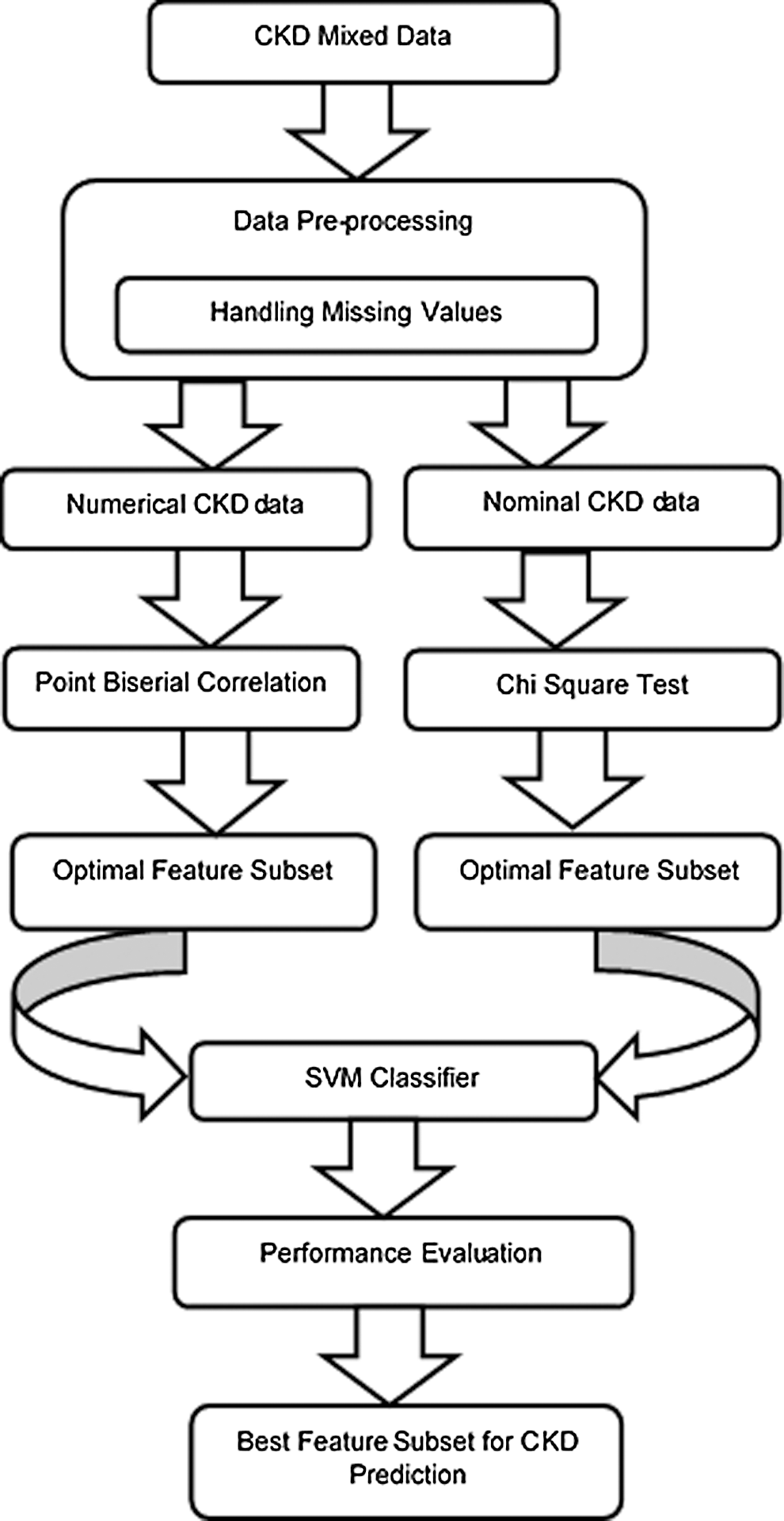
Figure 1: The proposed MDFS model for CKD prediction

4  Materials and Methods

4.1 Data Pre-Processing

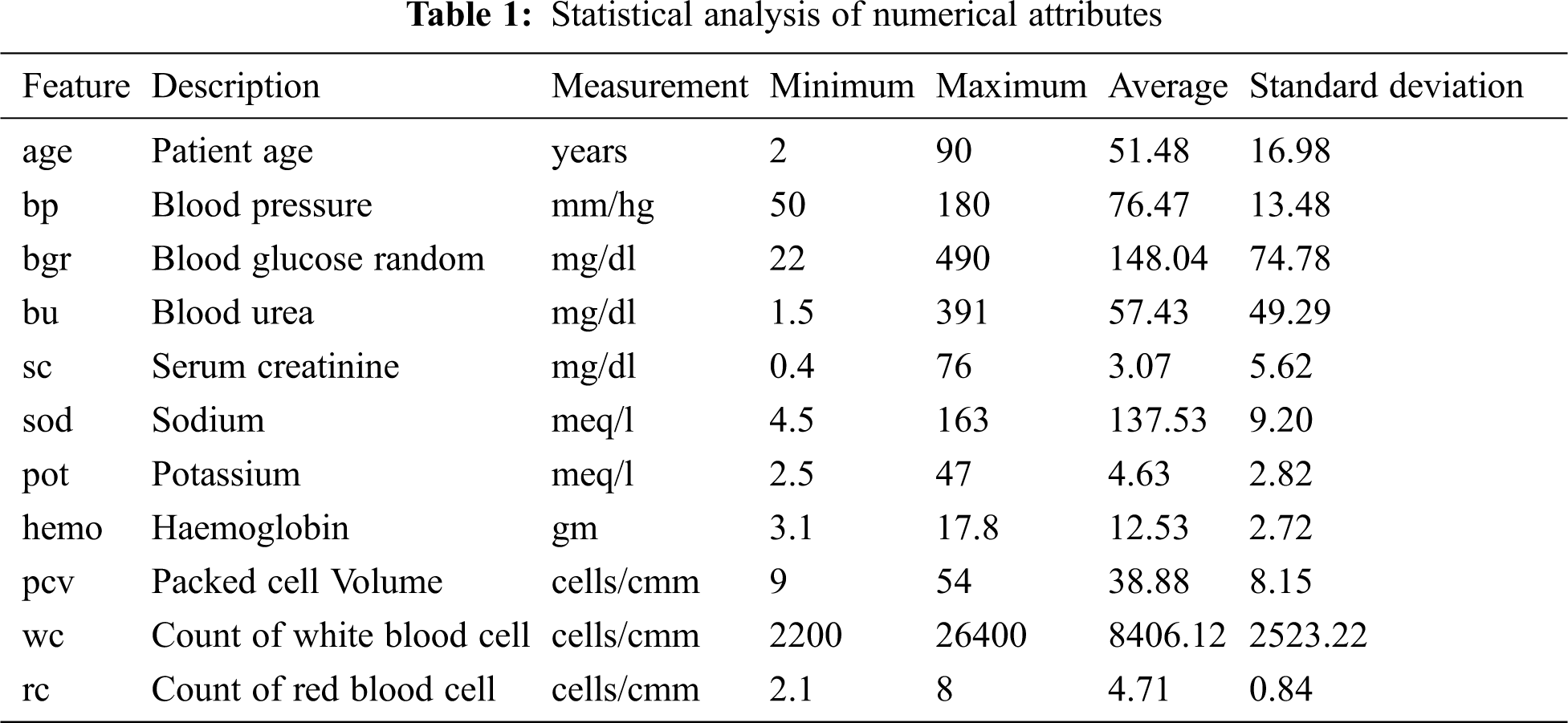
CKD data retrieved from the UCI repository is used in this experiment. This multivariate data was bestowed by a senior consultant nephrologist from Apollo hospitals, Tamilnadu, India [24]. The dataset consists of 25 features and 400 records, containing mixed data items of numerical and nominal data, as shown in Tabs. 1 and 2. Yes and no values are denoted as ‘Y’ and ‘N’. Normal and abnormal levels are indicated as ‘n’ and ‘an’. The presence and absence of cells are marked as ‘p’ and ‘np’. The 25th attribute is the class label with two classes CKD and not-CKD, representing patients with and without CKD by 250 instances and 150 instances. There are three categories of attributes present in the dataset: 1) Attributes related to the urine test, 2) Attributes related to the blood test, and 3) Attributes related to patient history. Besides, the dataset has missing values for a few attributes. Previous studies deal with missing values by removing the tuples that have missing values, ignoring the attributes with a larger percentage of missing values, or replacing the missing values with mean or median.

For proper selection of dominant features, CKD and not-CKD subjects are supposed to include all attributes initially. Then, the missing values are replaced with attribute mean for numerical features and with the more frequent label for nominal features. In addition, the dataset is split as a training and a testing dataset, where the mixed training data set is divided into subsets with numerical features and nominal features, respectively.

4.2 Feature Selection

Previous studies reveal that feature selection algorithms can be applied to the entire dataset irrespective of the data types in the dataset. Heterogeneous data are converted into homogeneous data using some discretization methods. But these conversions certainly lead to information loss and wrong analysis. The proposed system aims to identify the most dominant attributes that can aid in the early CKD prediction by involving separate feature selection algorithms on numerical and nominal data.

4.2.1 Chi-Square Test of Independence

The Chi-Square test is a test for independence between nominal variables, which determines whether the target class variable is dependent or independent of the input. If it finds independent, then input variables can be considered irrelevant and removed from the dataset. A Chi-Square test of independence χ2 compares two variables in a contingency table to see if they are related to each other. The advantage of using a Chi-square filter to process nominal features is to test the hypothesis about the distribution of observations in different categories like CKD and Not-CKD. It can help to assess whether two nominal variables from a single CKD data sample are independent of each other. The formula is given in Eq. (1).

χ2=∑(O−E)2/E (1)

where O is the observed frequency of values and E is the expected frequency of values.

The expected values are calculated in Eq. (2).

E=oc.orn (2)

where oc is marginal column frequency and or is marginal row frequency. The total sample size is denoted as n. The null (Ho) and alternative hypotheses (Ha) are formulated:

where Ho is the classification label not dependent on the nominal input feature, and Ha is the classification label dependent on the nominal input feature. The degree of freedom (df) is illustrated in Eq. (3).

df=(number of row−1)(number of column−1) (3)

4.2.2 Point Biserial Correlation

The Point Biserial correlation (rpb) coefficient is a measure to estimate the degree of relationship between a continuous variable and a naturally dichotomous nominal variable. It is an estimation of the coherence between the two variables. The function is described in Eq. (4).

r=pbM1−M0Snn1−n0n2 (4)

where M1 and M0 are the averages on the continuous variable X for all data points with dichotomous variable C with values 1 and 0, respectively. n1 and n0 represent the total numbers of data points in groups 1 and 2 separately. The total sample size is given as n.

4.2.3 Support Vector Machine

Support Vector Machine (SVM) ropes both regression and classification tasks and can handle multiple continuous and categorical variables. The classification process of SVM is to construct hyperplanes. Given labeled CKD training data, the SVM algorithm yields an optimal hyperplane that categorizes new instances. CKD training data consisting of n points form the Eq. (5).

((xi,yi)|xi∈RN,yi∈{−1,+1},i=1,...,n) (5)

where xi is the set of training tuples with the class label yi. Thus, the hyperplane is given in Eq. (6).

wT⋅x+b=0 (6)

where w is the weight vector and b is the scalar representing the bias.

H1:wT⋅x+b ≥ 1 ∀yi=+1 (7)

Any tuple that falls on or above H1 belongs to class +1, i.e., class CKD, as in Eq. (7), and any tuple that falls on or below H2 belongs to the class −1, i.e., class notCKD, as in Eq. (8).

H2:wT⋅x+b ≤ 1 ∀yi=−1 (8)

Eqs. (7) and (8) are represented in Eq. (9).

qyn(wTxn+b) ≥ 1, for all 1 ≤ i ≤ n (9)

Minimize the function in Eq. (9) to construct an optimal hyperplane in Eq. (10).

minw,b,ξ f(w,b,ξ)=‖w‖22+C∑n=1N⁡ξn (10)

subject to Eq. (11)

yn(wTxn+b) ≥ 1, for all 1−ξn,ξn>0 n=1,…,N (11)

The optimal hyperplane is given as the Lagrangian dual problem in Eq. (12).

maxLD(αi)=∑i=1lαi−12∑i=1lαiαjyiyj(xixj) (12)

subject to Eq. (13)

∑i=1mαiyi=0,αi>0,i=1,…,m (13)

where αi is the Lagrange multiplier.

The inner product between the training tuple x and the support vectors is calculated to make predictions in Eq. (14).

wT⋅x+b=∑i=1mαiyi(x x)+b (14)

5  Results and Discussion

The computed χ2 statistic of all nominal features calculated separately with the class label shown in Tab. 3 exceeds the critical value for a 0.05 probability level for the specific degree of freedom. The null hypothesis is rejected. It can be known from the test that the output feature is dependent on all nominal input features. To select the best features, a ranking method is employed, which ranks the input features in descending order based on their χ2 values.

Tab. 4 shows the χ2 values ranked in descending order. It can be seen from Tab. 4 that specific gravity is highly correlated with the classification label. Point Biserial correlation ranges from −1 to +1, which can be positive or negative. The calculated rpb between the numerical feature and the nominal class feature is shown in Tab. 5. The features are ranked by ignoring the negative sign from the computed rpb values. It is clear from the results that sod, hemo, pcv, and rc are negatively correlated with the classification feature, while other features are positively correlated. age, pot, and wc show a very small positive correlation level with class (CKD/notCKD). In this analysis, only five features with a high or moderate correlation level with class CKD/notCKD are selected. hemo, pcv, and rc are selected because they have a high negative correlation with class. bgr and bu are chosen because they have a moderate positive correlation with the class. The feature with the highest correlation in absolute value determines the most powerful influence on CKD prediction. The experiment is conducted by SVM as the classification algorithm with a poly kernel. Different sets of features shown in Tab. 6 are fed to SVM, and their classification accuracy is noted. Tab. 7 shows that the accuracy of SVM with set7 remains unchanged when the set8 features are added.

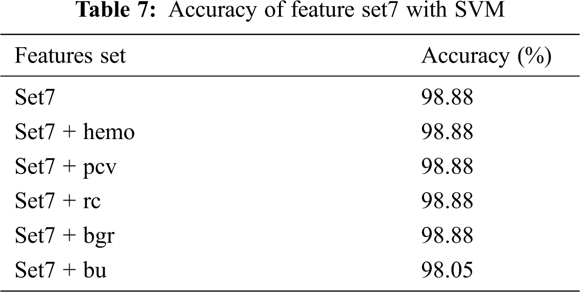
The set 7 feature subset is kept, and each feature from set8 is added with accuracy recorded. The addition of the top 5 numerical features, such as hemo, pcv, rc, and bgr, with set 7 does not increase or decrease the accuracy. But when bu is added to the set7 feature subset, the accuracy is dropped. The model is created by using a set 7 feature set. From the results, it is clear that set 7 produces the best accuracy of 98.8% when compared with other features set.

The MDFS model maintains the unique properties of numerical and nominal features without any feature transformation during feature selection. It guarantees no information distortion occurs due to discretizing the feature from one type to another.

The MDFS model is compared with other approaches by applying feature selection algorithms on the dataset and ignoring the importance of the feature type, as shown in Tab. 8. Besides, Tab. 9 shows that the proposed model outperforms previous works in terms of accuracy. The set of five features, such as sg, al, htn, dm, appet achieves a good prediction accuracy in classifying the CKD as healthy and unhealthy subjects.

6  Conclusion

In this paper, the MDFS model is built based on the idea of separate feature selection on nominal and numerical features. Point Biserial correlation is utilized to select numerical features, and a Chi-square filter is applied to determine nominal characteristics. Then, the SVM algorithm is employed to evaluate and choose the best feature subset. Both the feature types are selected independently and then merged based on the accuracy obtained by SVM. The set of five features sg, al, htn, dm, and appet identified as important predictors also includes the risk factors diagnosed by medical experts from mixed data without any data discretization during feature selections. Thus, the original properties of the medical data are preserved and guarantee no data distortion. The dominant attributes can help the patients and the medical practitioners to find a hint of CKD at the earlier stage. The predictions are limited to the size of the dataset. In the future, the work can be extended to identify the specific type of kidney disorder and its predictors.

Acknowledgement: The authors sincerely thanks to TopEdit team for providing Linguistic editing.

Funding Statement: The authors received no specific funding for this study.

Conflicts of Interest: The authors declare that they have no conflicts of interest to report regarding the present study.

This work is licensed under a Creative Commons Attribution 4.0 International License, which permits unrestricted use, distribution, and reproduction in any medium, provided the original work is properly cited.