DOI:10.32604/iasc.2022.019654
| Intelligent Automation & Soft Computing DOI:10.32604/iasc.2022.019654 | |
| Article |
An Optimized Scale-Invariant Feature Transform Using Chamfer Distance in Image Matching
1College of Computer Science and Informatics, Amman Arab University, Amman, Jordan
2Faculty of Information Technology, Al-Ahliyya Amman University, Amman, Jordan
3Faculty of Information Technology and Systems, University of Jordan, Aqaba, Jordan
4School of Business, University of Jordan, Amman, Jordan
*Corresponding Author: Issam Alhadid. Email: i.alhadid@ju.edu.jo
Received: 21 April 2021; Accepted: 20 June 2021
Abstract: Scale-Invariant Feature Transform is an image matching algorithm used to match objects of two images by extracting the feature points of target objects in each image. Scale-Invariant Feature Transform suffers from long processing time due to embedded calculations which reduces the overall speed of the technique. This research aims to enhance SIFT processing time by imbedding Chamfer Distance Algorithm to find the distance between image descriptors instead of using Euclidian Distance Algorithm used in SIFT. Chamfer Distance Algorithm requires less computational time than Euclidian Distance Algorithm because it selects the shortest path between any two points when the distance is computed. To validate and evaluate the enhanced algorithm, A data set with (412) images including: (100) images with different degrees of rotation, (100) images with different intensity levels, (112) images with different measurement levels and (100) distorted images to different degrees were used; these images were applied according to four different criteria. The simulation results showed that the enhanced SIFT outperforms the ORB and the original Scale-Invariant Feature Transform in term of the processing time, and it reduces the overall processing time of the classical SIFT by (41%).
Keywords: Image matching; image key points; SIFT; SURF; ORB; Chamfer distance algorithm; Euclidian distance algorithm
Digital images taken by digital cameras cover a wide range of objects around the world. These images are used for different purposes within different fields such as: medical field, design field, computer vision field, etc. Therefore, the computer vision field has rapidly developed by employing several methods to perform different tasks such as: image restoration, image clustering, image detection, and matching, etc. [1]. Image matching is the process of finding the shared correspondences between different images to check if the selected images have the same feature, object or describes the same thing [2]. Generally, image matching consists of three main steps as follows [3]:
• Feature detection.
• Feature location.
• Matching the features.
The image’s key points are extracted in the feature detection step. Those points might be located at the edges, corner, etc. (distinctive location), in other words, key points are the special points that describe the features of the image. As the digital images over the Internet become a valuable source of knowledge extraction, it can be used for different purposes. At the feature description step, the neighboring regions (pixels) around the key point are selected, then the descriptor for each region is identified. Lastly, at image matching step, the outputs of the previous step (the descriptors) are matched using similarity or distance measure such as: Euclidian distance [3]. Recently, different matching algorithms are proposed such as: SIFT [4], SURF [5], ORB [6], most of the proposed algorithms have common four key steps [7], as shown in Fig. 1.

Figure 1: Image matching steps [7]
On the other hand, Swaroop et al. [8] categorized the image matching techniques into four categories (Featured-based, Area-based, Template-based, Motion Tracking and Occlusion Handling).
Scale-Invariant Feature Transform (SIFT) is one of well-known image matching algorithms that work based on the local features in images [9]. Key points for each object are extracted in order to provide “feature description” of the object [4]. SIFT contains the following steps [10], as described in Fig. 2.
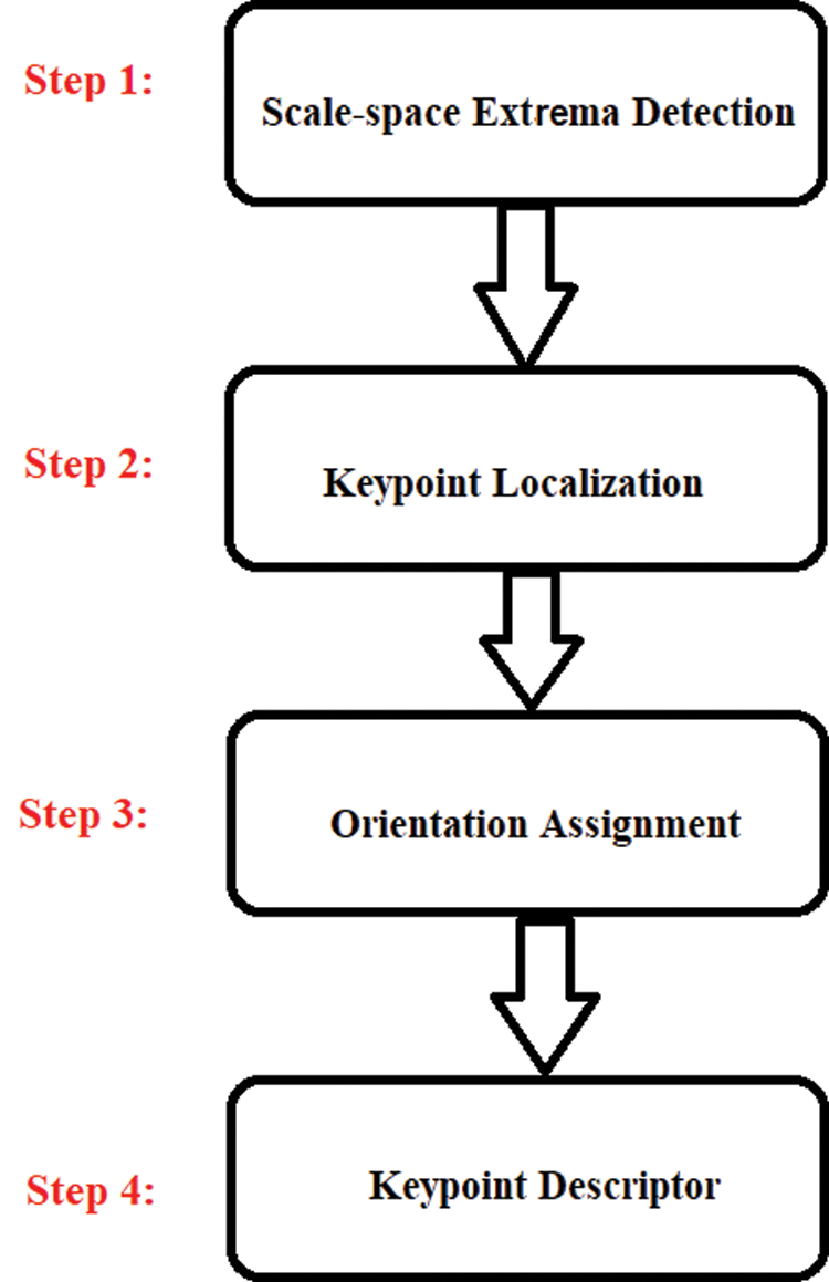
Figure 2: SIFT algorithm steps
In step 1, the key points are identified using Difference of Gaussian “DoF” over different scales of the image. In other words, the image’s scales and locations that differ the views of the same object are identified by searching the fixed features over all scales using scale space function. Different octaves from the original images are scaled to measure Gaussian value for each scale as shown in Fig. 3.
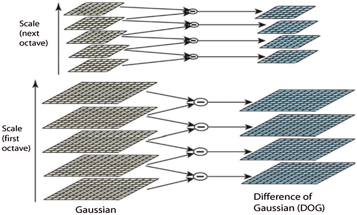
Figure 3: Gaussian and difference of Gaussian for different scales over different Octaves [10]
The scale space function is measured using Eq. (1) [10]:
where * indicates the convolution between two scales (x and y). G (x, y, σ) is the scale Gaussian, which is measured using Eq. (2) [10]:
Finally, in order to get the scale-normalized Laplacian of Gaussian, the difference of Gaussian is measured using Eq. (3) [10]:
After measuring the Difference of Gaussian, the local extrema detection step is started to find the minima and maxima of Difference of Gaussian. The original image is blurred by Gaussian several times with changing the σ value in order to compare the X point in the original image with the above and below scales as shown in Fig. 4.
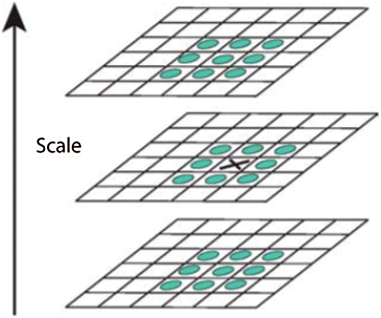
Figure 4: SIFT interesting points [10]
Each point (x) is compared with (3 × 3) neighbors in the same scale, then it is also compared with (3 × 3) in the high and low scale. So, we have 26 pixels to be compared with (x). If (x) is larger or smaller than the 26 pixels, (x) will be considered as SIFT interesting point. The number of scales that must be taken is 3 scales; because they captured the most of interesting points in 3 scales as the experimental analysis proves [10]. Hence, the number of interesting points is normalized by applying a thresholding on minimum contrast and eliminating the outliers (i.e, edge responses) using Hessian matrix or Harris detector. Then, the orientation assignment is applied to achieve rotation invariance using two functions, Magnitude (Eq. (4)), and Direction (Eq. (5)) respectively [10].
where m is the magnitude, θ is the orientation between two scales (x, y). As shown in Fig. 5, the orientation of each interest point is identified according to the direction of the interest point peak in the histogram. In case there is more than one peak, multi direction will be found. But, unique direction (i.e, unique peak) is generally exist for gradient.
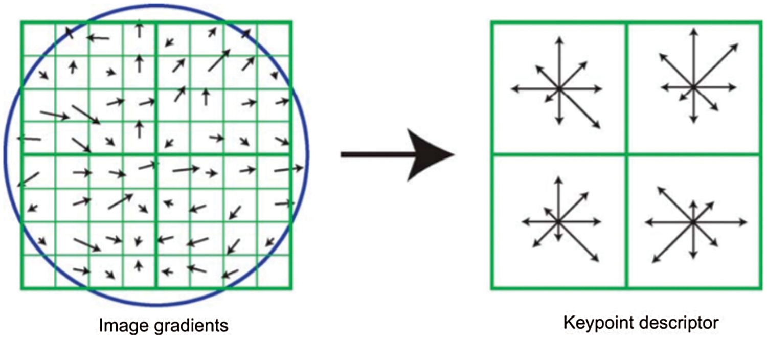
Figure 5: Image gradients and key points descriptors [10]
Once the SIFT descriptors are ready, the matching can be started according to the following scenario; For the original image, identify interesting points, then SIFT descriptors. For the matching image (i.e, testing image) identify interesting points, then SIFT descriptors. After that, distance measure (Euclidian distance) is used to measure the distance between the descriptors in the original and testing image. We look at the ratio distance between the best and the second-best matching, if the ratio is low, matching is good, else ambiguous matching. Regardless all of the SIFT advantages, it has main challenge and drawback in its processing time as it requires much of computational time especially in matching stage. This challenge minimizes the usage of SIFT in real time applications such as: image retrieval [11] and traffic light control [12].
Some researchers tried to enhance the performance of SIFT algorithm such as: Acharya et al. [13] used GPU on SIFT, also, [14] combined PCA-based local descriptors with SIFT algorithm, and Bay et al. [5] proposed SURF (Speeded Up Robust Features) to enhance the processing time of SIFT, but it still requires more enhancements in processing time without degrading the matching rate and its accuracy.
This paper proposes an enhanced SIFT algorithm for image matching based on Chamfer distance that reduces the processing time without degrading the matching rate. It also efficiently matches the images with different rotation degree, images with different intensity levels, images with different scaling levels and noisy image as well.
This research is organized as follows. Section 2 presents an overview of the related literature about the SIFT algorithm and other algorithms used for image matching and. Section 3, describes the proposed method, which covers preparing dataset, SIFT modification and evaluating the proposed algorithm. Section 4 discusses the results. Section 5 finally gives the research conclusions and the future directions.
In this section, a comprehensive review of the related works is presented to investigate the existing enhancements of the SIFT algorithm in image matching field.
Wang et al. [15] enhanced the processing time of the original SIFT by replacing the Euclidean distance measure by other distance measures, which are called (“the linear combination of city-block and chessboard distance”). The simulation results showed that the enhanced algorithm improves stability of algorithm and reduced the required time for performing matching process (processing time). Moreover, Daixian et al. [16] employ Chamfer distance as exhaustive search algorithm to improve SIFT algorithm during matching phase, this technique considers the matches in case of 0.8 difference between 1st and 2nd neighbors.
Chen et al. [17] used modified SIFT to be used in image mosaic method, the modified algorithm is combined with Canny feature edge detection. After extracting the features points using the original SIFT, 18-dimensional feature descriptor is used. Then, the features in 16-neighborhood of the Canny edge image. The RANSAC algorithm is used to compute the transformational matrix for the extracted features points. The image fusion algorithm is used to seamless mosaic. The simulation results indicate that the mosaic time is enhanced using the proposed method, as well as the root mean squared error is enhanced too.
Further, Abdollahi et al. [18] enhanced SIFT processing time by removing the duplicated interest points using threshold and grid ding. The experimental results on a drug database indicate that the enhanced SIFT reduce the processing time and the complexity as well. Moreover, the authors aimed to enhance the processing time of the original SIFT by dividing the original image to different regions, then applying the SIFT to each region. After that, deleting the duplicated matching points, and removing the wrong matching points in case of there are no matching points in the neighborhood regions or all of the key points are exceeded the threshold. To evaluate the proposed enhanced algorithm, using medical drugs database, they assessed it against the original SIFT according to running time to different stages including (orientation assignment, descriptor representation, matching phase, matching point set). The overall results showed that the proposed algorithm consumes less time in comparison with the original one.
In addition, Jin et al. [19] used enhanced SIFT to track of object and detecting of feature to video content. The enhanced technique is used as a part of tacking system because it provides a reliable object coordinate. Their approach compared against original SIFT using different genres of video. The evaluation results show that the modified SIFT reduces the processing time up to 5% compared with the original SIFT.
Hajano et al. [20] proposed a framework to improve the process of aligning two or more images of the same scene using the feature based and area-based methods. The framework uses different Filters and algorithms. In the preprocessing phase the Bilateral Filter is applied to remove the images noise from the reference image and the submitted image. In the next phase, the Speeded -Up Robust features (SURF) algorithm is used for feature detection while the NN (K-nearest neighbours) algorithm is used for matching the similar points between the two images. Later on, the Random sample consensus (RANSAC) algorithm is utilized to reducing the miss matches. In the finale phase, Template matching method is applied for the area-based matching to find the alignment points between the two images.
On the other hand, Bdaneshvar [21] proposed an enhanced SIFT algorithm. The descriptors of the improved algorithm use hue feature of key point to provide accurate matching. The experimental results indicate that the proposed algorithm decreases the computational complexity (as the number of key points is decreased) and decrease computational load in matching process (as the size of descriptors is decreased).
This section explains the main architecture of the proposed method of the enhanced SIFT algorithm in image matching, which matches images with different features within enhanced processing time. The main goal of this method is to optimize the processing time of the original SIFT algorithm when matching the images. Fig. 6 illustrates the main steps of the proposed method.
The Proposed Method, as Summarized in Fig. 6, Consists of the Following Stages
• Preparing datasets.
• Modified SIFT.
• Evaluating the proposed algorithm.
In this study, different datasets were used to test our proposed algorithm. These datasets were collected from different online resources to ensure its inclusivity (i.e, to cover all of the images’ features that may affect matching process including: scaling levels, rotation degree, intensity levels and noisy images).
The first dataset, consists of (100) images with different rotation degrees, was collected from dataset page of Middlebury Computer Vision to test the enhanced algorithm using images with different rotation degrees [22]. The dataset consists of (100) rotated images with different rotations’ coordination to be matched with the original images.
On the other hand, the second dataset is labeled faces in the wild home, which prepared by computer vision lab in University of Massachusetts [23]. It is used to test the enhanced algorithm using (112) original images to be matched with other (112) images (containing (65) scaled images with normal funneling, and (56) scaled images with deep funneling).
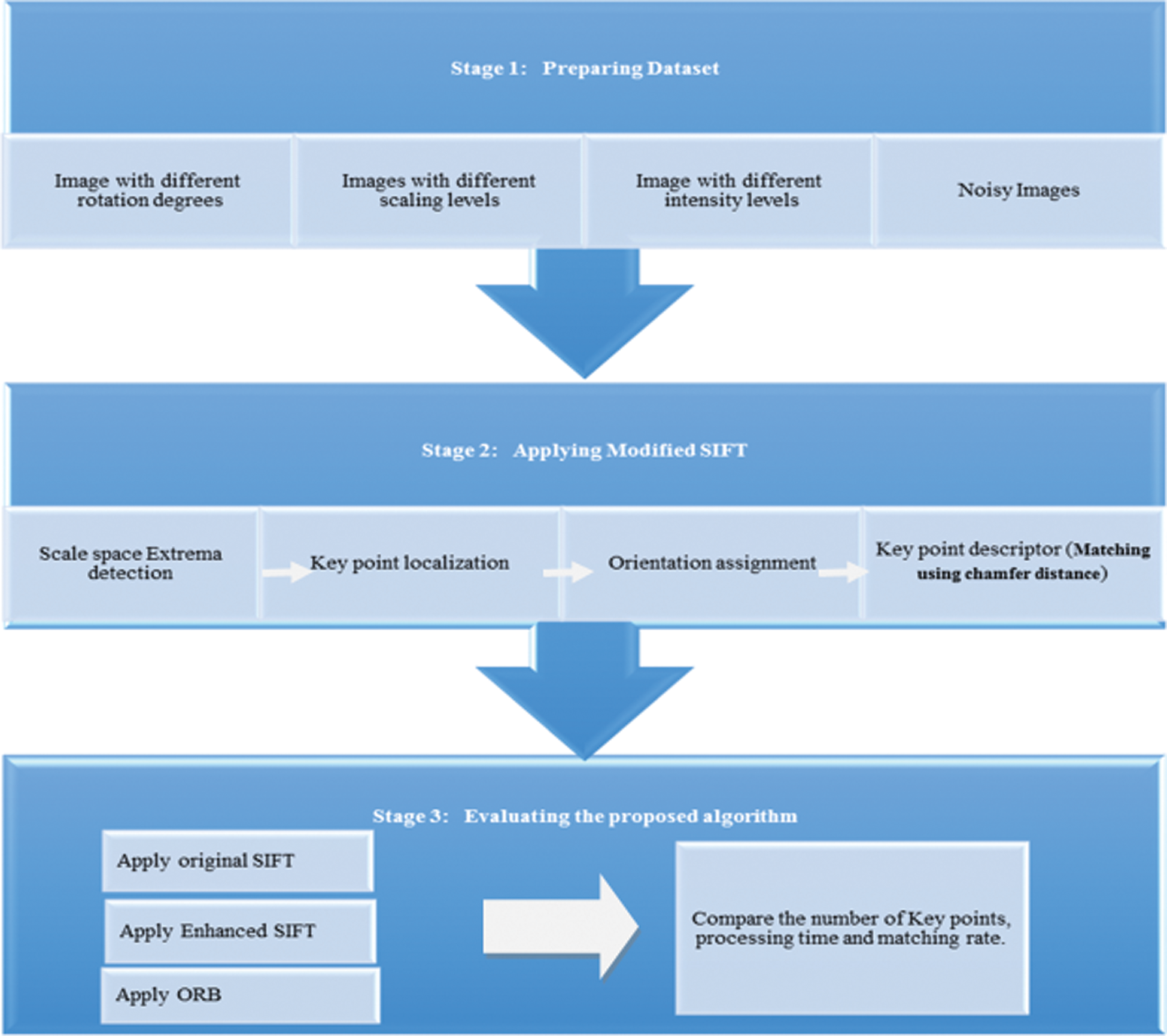
Figure 6: The proposed method
Further, the third dataset was collected from Berkeley Segmentation Dataset [24] to test the enhanced algorithm using images with different noise levels. The testing process was performed using (100) original images to be matched with other (100) noisy images (including (20) images affected by 5% Salt and Pepper noise, (20) images affected by 10% Salt and Pepper noise, (20) images affected by 20% Salt and Pepper noise, (20) images affected by 40% Salt and Pepper noise, and (20) images affected by 60% Salt and Pepper noise).
Finally, the fourth dataset was also collected from computer vision lab in University of Massachusetts [23] to test how the enhanced algorithm matches the images with different intensities. The testing process was performed using (100) original images to be matched with other (100) images with different intensities.
In details, the proposed algorithm follows the following steps when matching two images:
1. Scale Space Extrema detection: Images with different octaves from original image are created. The number of octaves depends on the size of original image. In detail, images in the first octaves employed to generate progressively blurred out images, then the original image is resized to half size and this resized image is transformed to be blurred images by Gaussian smoothing again. Original paper had suggested that 4 octaves and 5 blur levels are ideal.
2. Key point localization: In theorem, Laplacian of Gaussian (LOG) can be used to detect and extract edge and corner pixels based on the second order derivate of gray level in an image. Yet LOG is sensitive to noise, DOG (Difference of Gaussian) is used to approximate Laplacian of Gaussian. The images created in step 1 are utilized to calculate the difference between two images with consecutive scales. After DOG images are generated, edge and corner pixels can stand out. SIFT needs to find specific key points, but the points found in step 3 may be on the edge or with low contrast. For eliminating low contrast points, a threshold value can be used to filter low-contrast points. Additionally, two eigenvalues of Harris Matrix of each point can be used to decide whether the point is on the edge or not. If one eigenvalue has some large positive value and the other eigenvalue is a very small value, then this pixel (x, y) is an edge pixel. A lot of edge and corner pixels will be found after processing in step 2. This step will find candidate key points. For each point, eight points around it and nine points at the same location of its upper and lower image, total 26 neighbor points, will be considered to determine the candidate points. If the DOG value of this point is the maxima by comparing to its 26 neighbor points, then the point is viewed as a key point.
3. Orientation assignment: It will give every key point an orientation in this step. For each key point, its magnitude and orientation for all pixels around the key point will be calculated by the Eqs. (4) and (5). The first equation is magnitude of a pixel (x, y) and the second equation is orientation of a pixel (x, y), L (x, y) is the gray value of a pixel (x, y). A histogram is created for determining the key point orientation. When creating a histogram, it is recommended to divide 360 degrees into 8 regions. That means 0° ± 22.5°, 45° ± 22.5°, and so on. Then a 16
4. Key point descriptor matching using Chamfer distance: to improve the processing time of the original SIFT, Chamfer Distance Algorithm (CDA) is used instead of using Euclidian distance, because of Chamfer distance requires less computational time as it selects the shortest path between any two points. The chamfer distance between two points can be calculated according to Eq. (6):
where Ka and Kb are the movements numbers of a and b on the shortest route between two points (p, q) [25]. In other words, in case we have (3 × 3) image window, the distance using Chamfer is measured as mentioned below in Eqs. (7) and (8) [26].
Fig. 7 presents examples of different window size, in 3 × 3 windows, four points in the upper portion and four points in the lower portion are compared with the central point at the same time, in the same manner, in 5 × 5 window, eight points in the upper portion and eight points in the lower portion are compared with the central point at the same time, and so on [26,27].
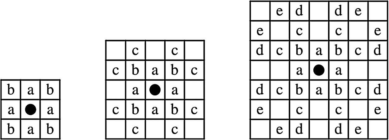
Figure 7: Examples of 3 × 3, 5 × 5 and 7 × 7 windows [26]
In a detail, the location of increments within 3 × 3, 5 × 5, 7 × 7 windows (i.e, the blank spaces) do not need to be tested because they are multiples of smaller increments, in other words, these points are not used (considered) during that pass of the algorithm. The pseudo code of the CDA is shown below, which summarizes the procedure of measuring the distance between the points in two passes (i.e, forward and backward).
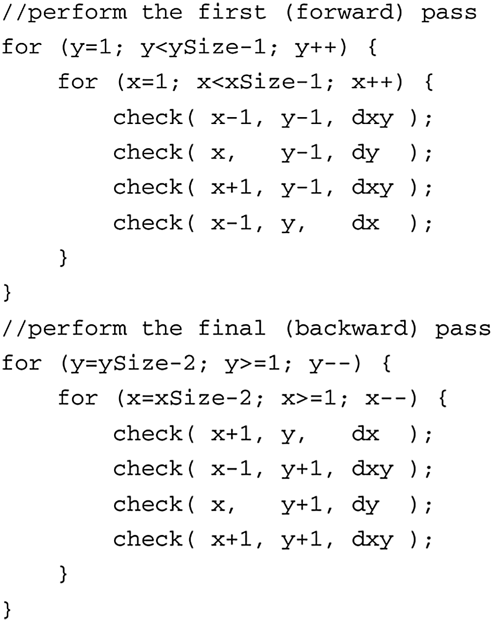
Fig. 8 Summaries the main flow (i.e, flowchart) of the enhanced algorithm.
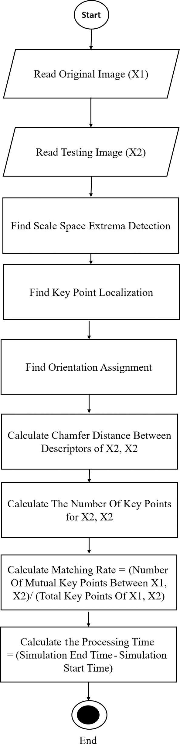
Figure 8: Enhanced algorithm flowchart
Different images dataset sets were collected and organized from different resources, as described previously in order to test the proposed technique with SIFT and ORB and to validate the paper assumption and to answer the paper questions.
4.1 Scenario 1: Applying Different Rotation Degrees
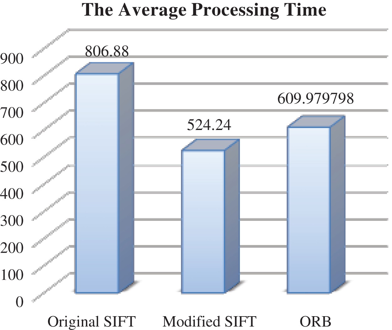
Figure 9: The average processing time- different rotation degrees
As mentioned before, the core optimization factor in this paper is the processing time that is required to match the images. As shown in Fig. 9 the simulation results showed that the modified SIFT reduces the required time for match the images, as it requires the least processing time (52424 ms), followed by ORB (60388 ms), then the original SIFT with (80688 ms). These results indicate that the modified SIFT reduces the processing time of the original SIFT by (35%) when applying it on rotated images.
4.2 Scenario 2: Applying Different Scales
Also, the processing time is enhanced using modified SIFT when applying it on the scaled dataset, as shown in Fig. 10. The modified SIFT outperforms (in term of processing time) the original SIFT and ORB, as modified SIFT required the least processing time (11013 ms), followed by the original SIFT with (21287 ms) and the ORB with (48758 ms) accordingly. Hence, the modified SIFT reduces the processing time of the original SIFT by (48.2%) when applying it on scaled images.
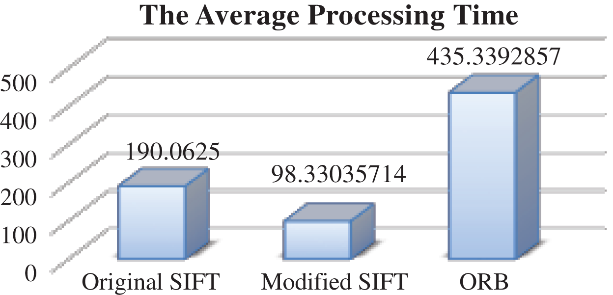
Figure 10: The average processing time-different scales
4.3 Scenario 3: Applying Different Noise Levels
The overall processing time and the average processing time when applying the matching algorithms on the noisy images’ dataset are presented below in Fig. 11. It is clear that the modified SIFT outperforms the original SIFT and ORB in term of processing time. The processing time that is required by modified SIFT is (42380 ms), but it is (54661 ms) the ORB and (77134 ms) for the original SIFT.
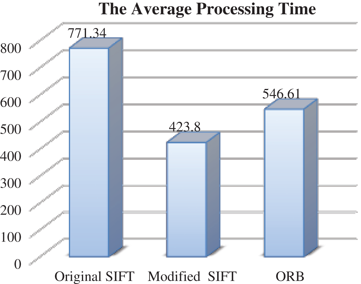
Figure 11: The average processing time-different noise levels
The modified SIFT improves the processing time of the original SIFT by (45%), and outperforms the original SIFT and the ORB in term of the processing time as shown in Fig. 12.
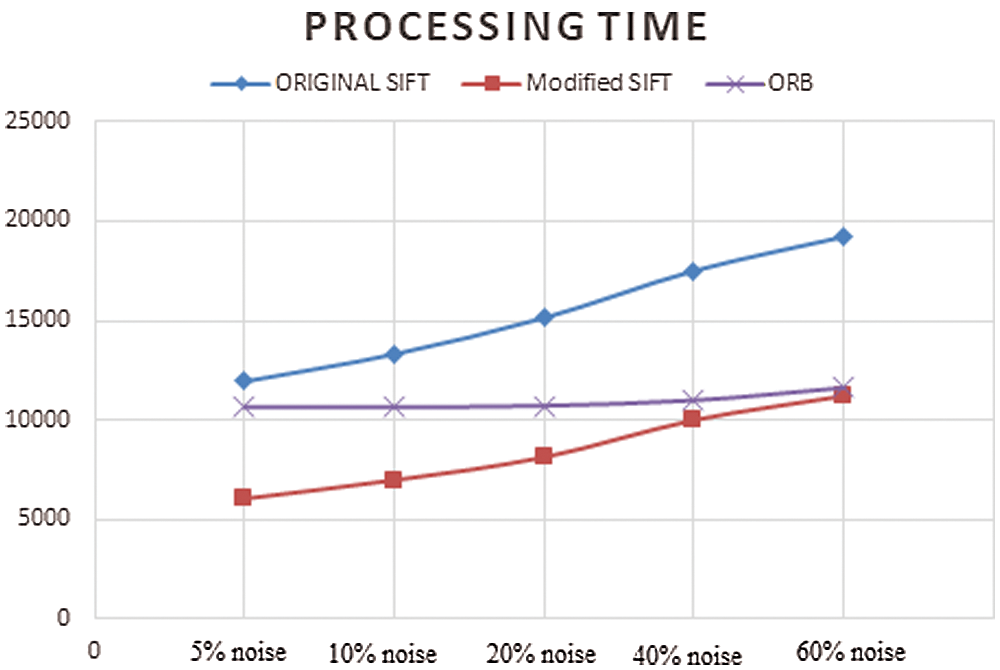
Figure 12: Comparison between image matching algorithms’ processing time- different noise levels
4.4 Scenario 4: Applying Different Intensities
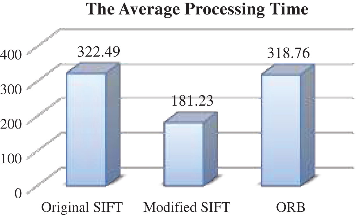
Figure 13: The average processing time-different intensities
Finally, as shown in Fig. 13, the simulation results showed that the modified SIFT reduces the required time for match the images, as it requires the least processing time (18123 ms), followed by ORB (31876 ms), then the original SIFT with (32249 ms). These results indicate that the modified SIFT reduces the processing time of the original SIFT by (43%) when applying it on rotated images.
SIFT is one of the most well-known image matching algorithms that attracts the researchers to perform their researches in this area due to its robustness. It can match the images with different rotations and different affine distortions and any other images’ modifications. Despite the robustness of the SIFT, it has some challenge related to its computational time. As it requires a long time, to some extent, to find and match the SIFT descriptors.
Various researchers enhanced the performance of the SIFT using different techniques or methods, but it still requires more enhancements in term of its processing time to be used in the real-time applications. This study proposes an enhanced SIFT algorithm in term of processing time by replacing the Euclidian distance by Chamfer distance without taking thresholds/conditions into considerations to efficiently match the images with different rotation degrees, different intensity levels, different scaling levels and the noisy images efficiently within short processing time where the time complexity of the Euclidian distance algorithm is O (log (a + b) while the time complexity of the Chamfer distance algorithm is O(N) which confirms the results of the proposed method [3,16]
Different datasets from different resources were used to evaluate the proposed algorithm against the original SIFT and the ORB, and the simulation results showed that the proposed algorithm generally outperforms the SIFT and the ORB in term of processing time when matching images with different rotation degrees, different intensity levels, different scaling levels and the noisy images.
Funding Statement: The authors received no specific funding for this study.
Conflicts of Interest: The authors declare that they have no conflicts of interest to report regarding the present study.
1. N. Jayanthi and S. Indu, “Comparison of image matching techniques,” International Journal of Latest Trends in Engineering and Technology, vol. 7, no. 3, pp. 396–401, 2016. [Google Scholar]
2. P. M. Panchal, S. R. Panchal and S. k. Shah, “A comparison of SIFT and SURF,” International Journal of Innovative Research in Computer and Communication Engineering, vol. 1, no. 2, pp. 323–327, 2013. [Google Scholar]
3. P. Mandle and B. Pahadiya, “An advanced technique of image matching using SIFT and SURF,” International Journal of Advanced Research in Computer and Communication Engineering, vol. 5, no. 5, pp. 462–466, 2016. [Google Scholar]
4. D. G. Lowe, “Object recognition from local scale-invariant features,” in Proc. of the Seventh IEEE Int. Conf. on Computer Vision, Kerkyra, Greece, pp. 1150–1157, 1999. [Google Scholar]
5. H. Bay, A. Ess, T. Tuytelaars and L. Van Gool, “Speeded-up robust features (SURF),” Computer Vision and Image Understanding, vol. 110, no. 3, pp. 346–359, 2008. [Google Scholar]
6. E. Rublee, V. Rabaud, K. Konolige and G. Bradski, “An efficient alternative to SIFT or SURF,” in Proc. of the Int. Conference on Computer Vision, Barcelona, Spain, pp. 2564–2571, 2011. [Google Scholar]
7. W. Song and H. H. Liu, “Comparisons of image matching methods in binocular vision system,” in Proc. of the Int. Conf. on Cyberspace Technology, Beijing, China, pp. 316–320, 2013. [Google Scholar]
8. P. Swaroop and N. Sharma, “An overview of various template matching methodologies in image processing,” International Journal of Computer Applications, vol. 153, no. 120, pp. 8–14, 2016. [Google Scholar]
9. U. M. Babri, M. Tariq and K. Khurshid, “Feature based correspondence: A comparative study on image matching algorithms,” International Journal of Advanced Computer Science and Applications, vol. 7, no. 3, pp. 206–210, 2016. [Google Scholar]
10. D. G. Lowe, “Distinctive image features from scale-invariant keypoints,” International Journal of Computer Vision, vol. 60, no. 2, pp. 91–110, 2004. [Google Scholar]
11. P. Chhabra, N. K. Garg and M. Kumar, “Content-based image retrieval system using ORB and SIFT features,” Neural Computing and Applications, vol. 32, no. 7, pp. 2725–2733, 2020. [Google Scholar]
12. P. Choudekar, S. Banerjee and M. K. Muju, “Real time traffic light control using image processing,” Indian Journal of Computer Science and Engineering, vol. 2, no. 1, pp. 6–10, 2011. [Google Scholar]
13. A. Acharya and R. V. Babu, “Speeding up SIFT using GPU,” in Proc. of the Fourth National Conf. on Computer Vision, Pattern Recognition, Image Processing and Graphics, Jodhpur, India, pp. 1–4, 2013. [Google Scholar]
14. Y. Ke and R. Sukthankar, “PCA-SIFT: A more distinctive representation for local image descriptors,” in Proc. of the IEEE Computer Society Conf. on Computer Vision and Pattern Recognition, Washington, DC, USA, pp. 2, 2004. [Google Scholar]
15. X. Wang and W. Fu, “Optimized SIFT image matching algorithm,” in Proc. of the IEEE Int. Conf. on Automation and Logistics, Qingdao, China, pp. 843–847, 2008. [Google Scholar]
16. Z. Daixian, “SIFT algorithm analysis and optimization,” in Proc. of the Int. Conf. on Image Analysis and Signal Processing, Zhejiang, China, pp. 415–419, 2010. [Google Scholar]
17. Y. Chen, M. Xu, H. L. Liu, W. N. Huang and J. Xing, “An improved image mosaic based on canny edge and an 18-dimensional descriptor,” Optik-International Journal for Light and Electron Optics, vol. 125, no. 17, pp. 4745–4750, 2014. [Google Scholar]
18. A. Abdollahi, A. T. Targhi and M. M. Dehshibi, “Optimized SIFT: An efficient algorithm for matching medical products images,” in Proc. of the Tenth Int. Conf. on Digital Information Management, Jeju, Korea (Southpp. 160–163, 2015. [Google Scholar]
19. R. Jin and J. Kim, “Tracking feature extraction techniques with improved SIFT for video identification,” Multimedia Tools and Applications, vol. 76, no. 4, pp. 5927–5936, 2017. [Google Scholar]
20. S. Hajano, B. Naz and S. Talpur, “Area and feature based image registration using template matching and SURF algorithm,” in Proc. of the Int. Conf. on Computational Sciences and Technologies, Jamshoro, Pakistan, pp. 109–113, 2020. [Google Scholar]
21. M. Bdaneshvar, “Scale invariant feature transform plus hue feature,” in Proc. of the Int. Conf. on Unmanned Aerial Vehicles in Geomatics, Bonn, Germany, pp. 27–32, 2017. [Google Scholar]
22. D. Scharstein, H. Hirschmüller, Y. Kitajima, G. Krathwohl, N. Nešić et al., “High-resolution stereo datasets with subpixel-accurate ground truth,” in Proc. of the German Conf. on Pattern Recognition, Münster, Germany, pp. 31–42, 2014. [Google Scholar]
23. G. B. Huang, M. Mattar, T. Berg and E. Learned-Miller, “Labeled faces in the wild: A database for studying face recognition in unconstrained environments,” in Workshop on Faces in Real-Life Images: Detection, Alignment, and Recognition, Marseille, France, pp. 1–14, 2008. [Google Scholar]
24. D. Martin, C. Fowlkes, D. Tal and J. Malik, “A database of human segmented natural images and its application to evaluating segmentation algorithms and measuring ecological statistics,” in Proc. of the Eighth IEEE Int. Conf. on Computer Vision, Vancouver, Canada, pp. 416–423, 2001. [Google Scholar]
25. S. Marchand-Maillet and Y. M. Sharaiha, “Euclidean ordering via chamfer distance calculations,” Computer Vision and Image Understanding, vol. 73, no. 3, pp. 404–413, 1999. [Google Scholar]
26. D. G. Bailey, “An efficient Euclidean distance transform,” in Proc. of the Int. Workshop on Combinatorial Image Analysis, Berlin, Heidelberg, pp. 394–408, 2004. [Google Scholar]
27. G. J. Grevera, Distance transform algorithms and their implementation and evaluation. in The Deformable Models, 1st ed., vol. 1. New York, NY: Springer, pp. 33–60, 2007. [Google Scholar]
 | This work is licensed under a Creative Commons Attribution 4.0 International License, which permits unrestricted use, distribution, and reproduction in any medium, provided the original work is properly cited. |