Intelligent Automation & Soft Computing DOI:10.32604/iasc.2022.019811
Article

Intelligent Audio Signal Processing for Detecting Rainforest Species Using Deep Learning

Rakesh Kumar1, Meenu Gupta1, Shakeel Ahmed2,*, Abdulaziz Alhumam2 and Tushar Aggarwal1

1Department of CSE, Chandigarh University, Punjab, India
2Department of Computer Science, College of Computer Sciences and Information Technology, King Faisal University, Al-Ahsa, 31982, Saudi Arabia
*Corresponding Author: Shakeel Ahmed. Email: shakeel@kfu.edu.sa
Received: 26 April 2021; Accepted: 14 June 2021

Abstract: Hearing a species in a tropical rainforest is much easier than seeing them. If someone is in the forest, he might not be able to look around and see every type of bird and frog that are there but they can be heard. A forest ranger might know what to do in these situations and he/she might be an expert in recognizing the different type of insects and dangerous species that are out there in the forest but if a common person travels to a rain forest for an adventure, he might not even know how to recognize these species, let alone taking suitable action against them. In this work, a model is built that can take audio signal as input, perform intelligent signal processing for extracting features and patterns, and output which type of species is present in the audio signal. The model works end to end and can work on raw input and a pipeline is also created to perform all the preprocessing steps on the raw input. In this work, different types of neural network architectures based on Long Short Term Memory (LSTM) and Convolution Neural Network (CNN) are tested. Both are showing reliable performance, CNN shows an accuracy of 95.62% and Log Loss of 0.21 while LSTM shows an accuracy of 93.12% and Log Loss of 0.17. Based on these results, it is shown that CNN performs better than LSTM in terms of accuracy while LSTM performs better than CNN in terms of Log Loss. Further, both of these models are combined to achieve high accuracy and low Log Loss. A combination of both LSTM and CNN shows an accuracy of 97.12% and a Log Loss of 0.16.

Keywords: Audio classification; spectrogram; CNN; LSTM; multi-class log loss

1  Introduction

A long time ago (i.e., more than 500 lakh years ago), Rainforest formed after tropical temperatures dropped down drastically when the Atlantic Ocean had widened enough to provide a warm, moist climate to the Amazon basin [1]. Origin of the rainforest dates to the Eocene era. There are a large variety of people who have always lived only in the Rainforest, many of them work as farmers but not on a large scale, they usually trade the products which have an excessive cost outside the forest which includes honey, hides, and feathers [2]. Rainforest includes a large variety of species which accounts for 50% of the world’s total species [3]. Rainforests consist of a large variety of fauna, including mammals, reptiles, amphibians, birds, and invertebrates. Reptiles include snakes, turtles, chameleons, some of them may be dangerous and their attack can even result in a life-threatening situation. According to the researchers, more than half of all biotic species are only found in the rainforest. Not only this, but researchers believe that there is a large variety of species that is still undiscovered and a continuous process is going on to find those species. Earlier, people have tried to become experts in all kinds of species by going through the training program for a forest ranger. But there are many species which are only found in tropical rainforest and hence few people know about them and so, even forest rangers are being deprived of this type of training. It takes years of real-world experience to become an expert but machine learning can help in automating this process and not let us worry about knowing all bits and pieces of every species. A model can be built that can act as a companion and recognize every species that is around us while roaming in a forest.

The sign of climate change and habitat loss can be achieved by the presence of rainforest species. Recognizing these species visually is not as simple as by hearing them, it’s important to use acoustic technologies that can work on a global scale. Machine learning techniques can supply real-time information and it could enable early-stage detection of human impacts on the environment. This result could drive more effective conservation management decisions [4]. To train a model on audio data, audio was needed to be somehow converted to mathematical numbers, to counter this issue, this paper uses a library called Librosa [5] which converts any given audio signal to time series format (Amplitude vs. time), Amplitude represents how loud an audio signal is, while thinking intuitively it certainly doesn’t seem reasonable to use loudness of sound to distinguish between different species but Amplitude can be converted to a frequency domain which seems a good preprocessing technique to be used.

This paper is further classified into different sections and sub-sections which explain various stages of this paper. Section 2 includes a high-level overview of work that has already been done in audio signal processing by different researchers. Next, the methodology used in this paper with data collection and all the necessary preprocessing steps are discussed in Section 3. The next Section 4 shows result formulation and evaluation with the help of LSTM and CNN. Finally, Section 5 gives the conclusion and future scope of the work.

2  Related Work

2.1 Criteria and Alternatives Selection

This section describes work related to Audio Classification and other preprocessing techniques for an audio signal that has been used by other researchers to improve results.

In [6], authors presented a method for data augmentation, they named it SpecAugment. It was combined with the inputs of the features of the network. The author proposed an augmentation policy that was quite different from traditional augmentation techniques and included the blocking of masks of time steps and frequency channels. With the help of these augmentation techniques, authors were able to achieve superior performance on some of the popular audio datasets. In [7], the authors presented a technique for removing noise from audio signals that included a combination of two processes carried out in frequency domain and time domain (Amplitude). They input the raw audio signal to a deep neural network and the resultant learning was only partially good, the prediction of the network helped to separate the noise from the audio signal. In [8], the authors used Libri-Light dataset to use its unlabeled audio samples to obtain superior results using semi-supervised learning given its massive developments in recent time. They used pre-trained giant Conformer models that were pre-trained with the weights of w2vec, with the help of this they performed student training with noisy data using augmentation techniques. Similarly, [9] also used semi-supervised learning, the authors first trained a Convolutional neural network for weak supervised learning on audio samples. Their methods were quite usual as they carried out the training, after that they demonstrated the effects of wrongly labeled data on semi-supervised learning. They also did a feasibility study and analyzed the cost of getting their hands on the weakly labeled data so that they do not have to produce it manually and compared it against a dataset that has been labeled by experts manually.

In [10], the authors worked on a dataset that was manipulated with some samples that did not belong to any class because of a labeling error. They proved that using those OOD (out of distribution) samples by separating them from the dataset can affect the training of the model in an effective way. They built a classifier that used data that was confirmed not to be from OOD samples. For separating OOD samples from the original dataset and label them again with correct labels, they used a small set of data for this experiment. They used a popular dataset that had some OOD samples and their results were promising and outperformed all the earlier work. In [11], authors proposed a neural network that worked on Time domain signals rather than frequency domain, in this they used the time domain signal to train encoder-decoder architecture and separated the non-negative outputs of the encoder. Using this, they were able to discard the frequency breakdown process and it helped to tear down the problem of separation to getting the masks of source on the outputs of the encoder which is later used by the decoder. Their techniques were even more powerful than the current SOTA for different types of Audio signal algorithms, they also brought down the cost of the project and the latency by a significant margin. There may be some cases where multiple voices are there in the audio signal at the same time, in [12], the authors proposed a method that can separate the audio signal which has multiple voices at the same time. The method used gates just like LSTMs and these gates were trained to separate each voice from the incoming audio signal while keeping the number of sources the same. They trained a separate network for each source and then used it to get the original number of sources in each sample. In [13], authors focused on using a deep neural network to perform the same task in the waveform domain, which separated the speakers within a region of θ ± w/2, where θ stands for angle of interest and w stands for window size. By decreasing w exponentially, they performed a binary search to separate all speakers with log-based time complexity. This technique was able to separate any number of speakers during test time even more than what it has seen during training. They showed that it achieved SOTA performance for speaker separation even when there is extremely high background noise.

In [14], authors discussed a network that they used to compete in Task 5 of the 2020 DCASE challenge. They used a neural network based on urban sound tagging which uses log spectrogram and time, location-based features as input, and outputs multilabel prediction vector. In [15], the author proposed a 1D convolution-based model, Jasper, which also included skip connection, Dropout layer, Batch Normalization layer, and ReLu as activation unit. To get better performance on training, they experimented with an optimizer that worked layer by layer, NovoGrad. With this usage, they proved that this network performs better than some of the complex networks. 54 layers of convolutions were used in their deepest neural network. This network allowed them to get WER of 2.95% using a decoder based on beam-search combined with an external NLP model and WER of 3.86% with a decoder based on a greedy algorithm. In [16], the authors proposed ContextNet, which used an encoder based on a fully connected convolution layer that internally used context information by adding squeeze-and-excitation modules. Also, they introduced a technique for scaling that standardize the ContextNet parameters and achieved a good balance between required resources and performance. They demonstrated that on some of the popular dataset, their architecture performed exceptionally good by showing a word Error Rate (WER) of 2.1%/4.6% without exterior NLP model, 2%/4% with LM (Language Model), and 3%/6.98% with only 10 Million parameters on the clean/noisy test sets. This compared to the best previously published model of 2.1%/4.5% with LM and 3.94%/11.33% with 20 Million parameters.

In [17], the authors experimented with diverse types of Convolution based network to perform classification on a dataset which consisted of 700 Lakh of videos for model training which included more than 30k labels based on the level of video. They used FCDNNs, Inception, ResNet, VGG, and AlexNet. They examined the size of unique label and dataset for training models, concluding that certain model designed especially for image-related task performs incredibly well on the classification of audio signals and a bigger dataset for training helped to improve the results. In [18], the authors presented the CLNN (Conditional Neural Network) and the MCLNN (Masked Conditional Neural Network), specifically made for recognizing time-based signals. The conditional neural network took into account the time-based behavior of the audio signal and the Masked architecture combined with Conditional architecture using 0/1 mask to retain the features based on locality and automated the process of exploring analogously combining features to crafting most important variables through the hand for the task. Their experiments achieved a high-class performance.

Based on above discussed different researcher views about the audio signals, it has been shown that a lot of work needs to be done in this area but there are some challenges and in this paper, techniques like frequency domain conversion of audio signals and combination of two types of models have been used to improve the results.

3  Methodology of Research

In this section, dataset collection, preprocessing steps have been discussed with performance metrics used for further evaluation.

3.1 Dataset

The dataset used in this paper collected from a Kaggle Competition repository [4], where it was explained that this data was collected through a device which along with recording audio also detected which species voice was there in the audio. Tab. 1 displays the distribution of each species for training and testing.

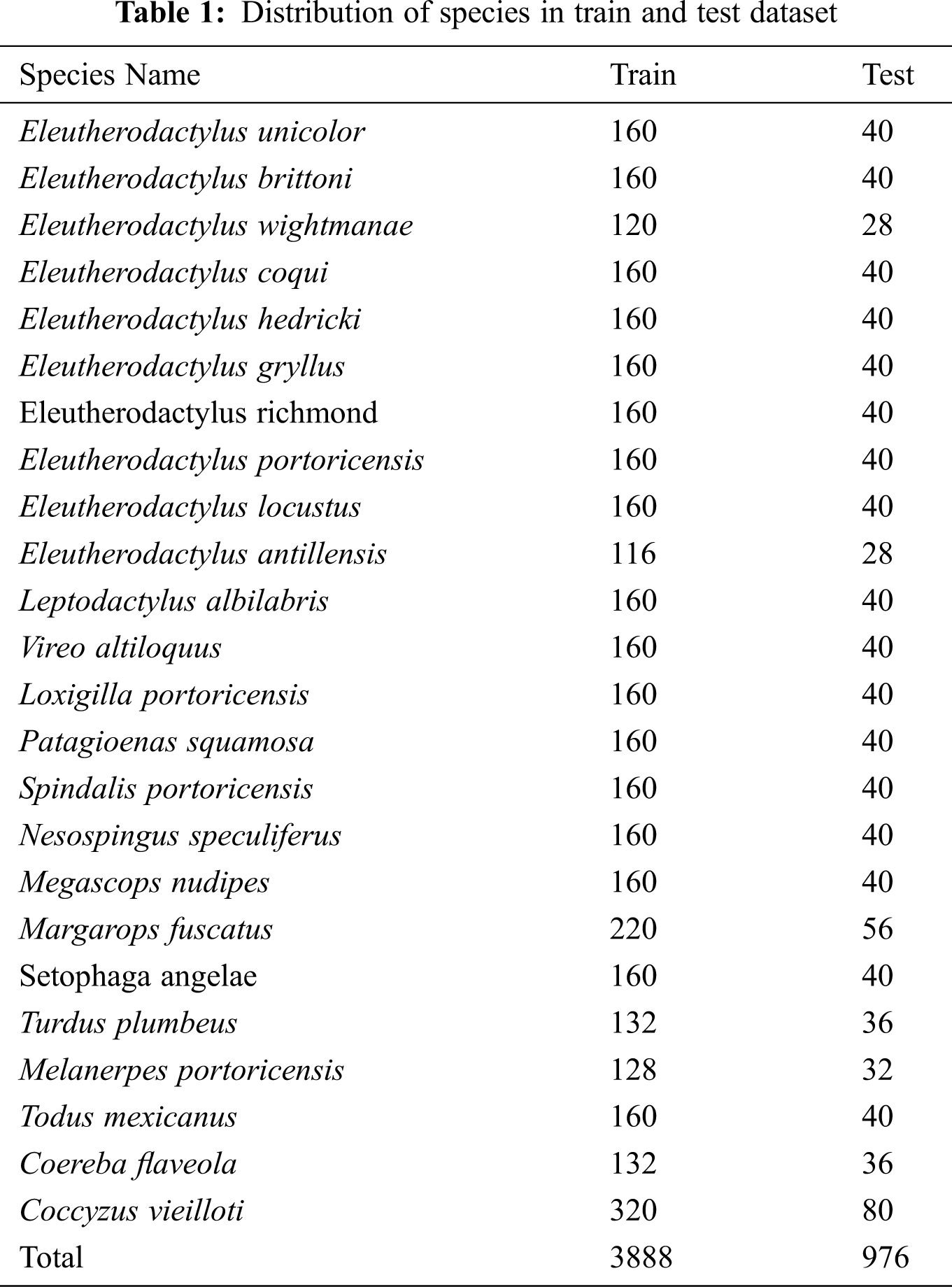
A total of 4727 audio signals were recorded and later this data was manually checked by experts and for ~1100 of these audio files, they found that their device detected correct species and information for these ~1100 files were stored in a separate file which contains the name of the audio file, species which is present in the audio, maximum and minimum frequency of the audio and the time at which a species was heard in that audio file. For the remaining ~3600 files, experts found that species detected by their device was not true and all the information for these audio files was stored in a separate file. Both of the files are provided in the competition repository and all the audio recording files are in .flac format which is used for storing lossless digital signal and as a result, this makes complete data of 17 GB+ size. Audio files are sampled at 44100 Hertz, as correct species label is only provided for ~1100 files so, in this work, ~1100 files are used and later preprocessing techniques like augmentation and time-based slicing are used to increase the size of data which increases total data samples to 4864, out of these files, 3888 files are used for training and 976 files are used for testing.

3.2 Model Formulation

To implement a deep learning model, all the files were loaded using Librosa and then sliced according to the time at which a species is heard (i.e., let’s say audio files is of 60 s and a species is heard in the audio at 5-8 s then audio signal at that particular time was separated to use it for further steps.), but it should not be very precise for the slice time as it may not help the model in generalization. So, in addition to the slicing audio file according to the given time, 0.2 s was also added at the start and beginning.

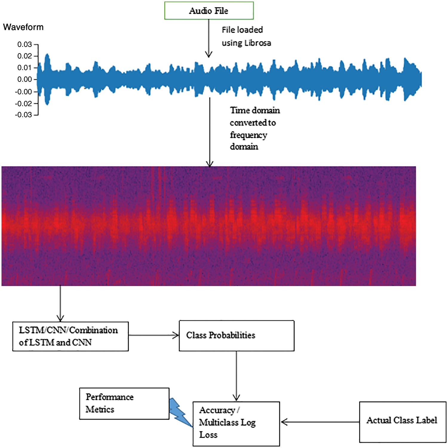
Figure 1: Proposed model for rainforest species audio detection

Train and test split was performed and new labels were also generated as each file was loaded twice. Data Augmentation techniques like time stretch and pitch shift were also used based on uniform distribution to make the model more generalized and new labels were also generated according to the data augmentation. Random numbers with uniform distribution were generated to decide which augmentation technique should be applied to a sample. Every audio signal was needed to be of the same length. According to the data analysis, there is very much difference in length of different audio files, the maximum length of an audio file was checked and all other signals were post padded accordingly. After that to perform data normalization, mean and standard deviation were computed. Fig. 1 shows the proposed model for Rainforest Species Audio Detection.

3.2.1 Long Short Term Memory

This section uses LSTM analysis for the considered dataset. This model is created in such a way that it captures sequential info of frequency of the sound of a species (LSTM layer with 50 units) along and then calculates average frequency over the sample (Global Average Pooling). Next, a dense layer with 32 units is used in the network and then a Dropout layer is also applied to regularize the model which can prevent overfitting and underfitting. The final layer of the model is a Dense layer that uses Softmax as an activation unit to generate the final prediction. Weights for this model were initialized randomly and the model was trained for 100 epochs. Fig. 2 shows the above-discussed neural network architecture based on LSTM.

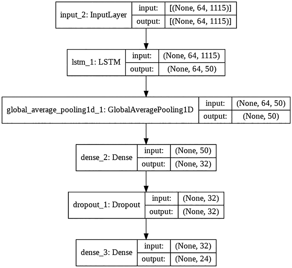
Figure 2: LSTM based architecture

3.2.2 Convolution Neural Network

This section uses CNN analysis for the considered dataset. This model tries to capture patterns in frequency based on sliding window using Kernel and strides through a convolutional layer with 24 filters and 5 kernels. Next, it uses a MaxPooling layer with 2 strides to get the maximum frequency, this process is repeated two times and then a GlobalAveragePooling layer is used to get the average frequency. Later, a Dropout layer is also applied to regularize the model which can prevent overfitting and underfitting, and then the final layer of the model is a Dense layer with 24 units which uses Softmax as an activation unit to generate the final prediction. Weights for this model were initialized randomly and the model was trained for 100 epochs. Fig. 3 shows the above-discussed architecture based on CNN.

3.2.3 Combined Approach for CNN and LSTM Analysis

In this section, both CNN and LSTM models are combined. For this, the input layer has been connected to two different layers, one is a Convolutional layer with 24 filters and 5 kernels and the other is an LSTM layer with 50 units. After this, the same layers are used as used in the previous two models. Next, the Dense layer of CNN and LSTM has been combined and a Dropout layer with a 0.3 rate is used to prevent overfitting and underfitting and then the final layer of the model is a Dense layer with 24 units which uses Softmax as an activation unit to generate the final prediction. Weights for this model were initialized randomly and the model was trained for 300 epochs. Fig. 4 shows the above discussed neural network architecture.

3.2.4 Performance Metrics Used: Multiclass Log loss/ Categorical Cross Entropy

As probabilities were to be predicted instead of actual class labels, using Multiclass Log Loss would be a better option instead of using accuracy [19], which can be defined as -ve average of log (probability of actual class label). Eq. (1) discusses about the formulation of Multiclass Log Loss.

F=−1n∑iN⁡∑jM⁡yij∗Ln(pij)=∑jM⁡(−1N∑iN⁡yij∗Ln(pij)) (1)

where F is loss, pij is the probability output by the classifier, yij is the binary variable (1 if expected label, 0 otherwise), N is the number of samples, M is the number of classes.

OR

Loss=−1N(∑iN⁡log⁡(P)) (2)

where P is the probability of the actual class label and N is the number of samples.

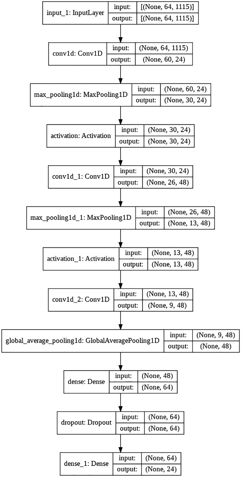
Figure 3: CNN based architecture

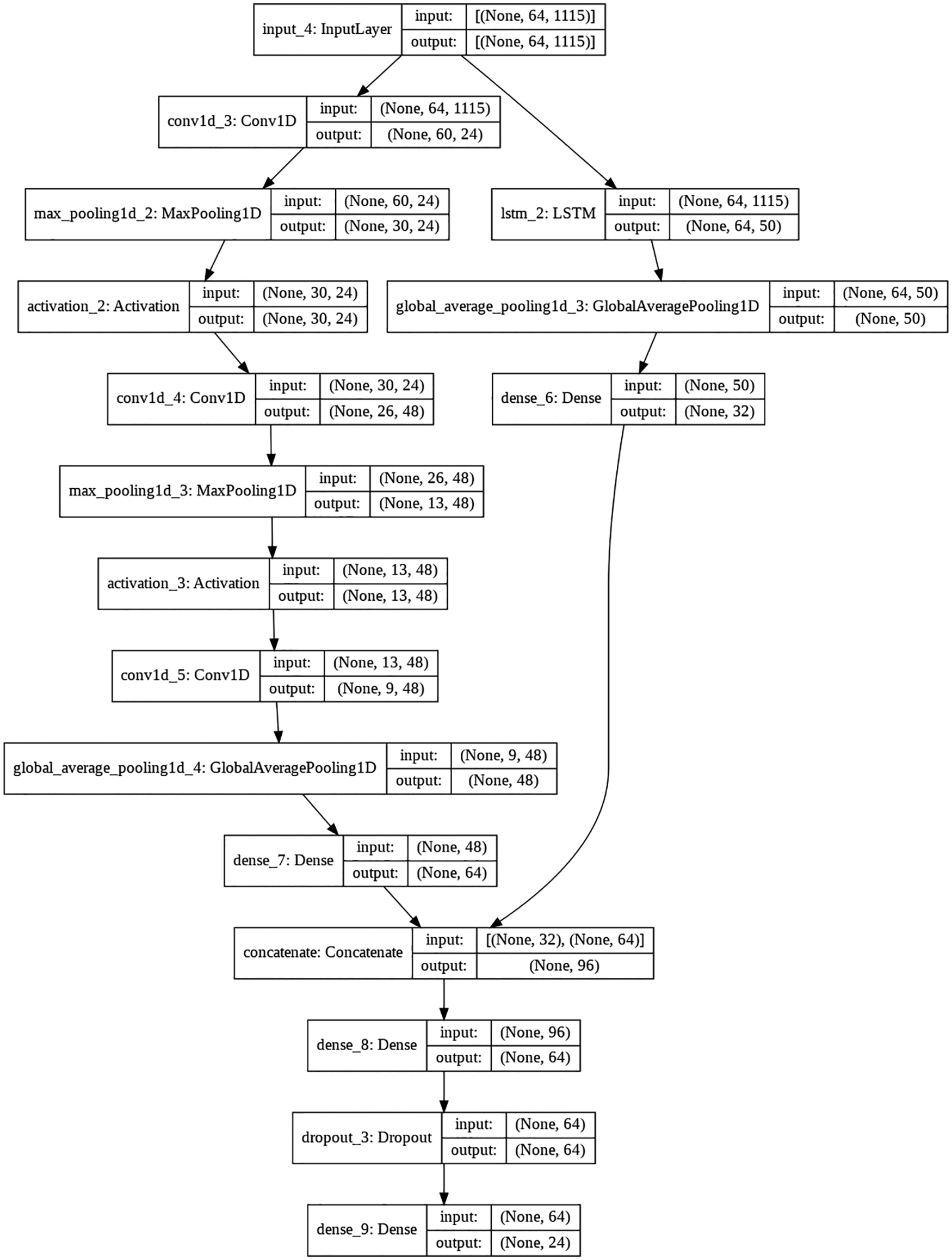
Figure 4: Proposed architectural model

3.3 Proposed Algorithm

This paper uses a combination of LSTM and CNN. The following steps describe the end-to-end working of algorithm and model architecture along with the purpose of each part of the architecture. The model can be divided into the following 5 steps:

Step 1- Preprocessing

a) Load audio file using Librosa at a sampling rate of 44100 Hertz

b) Convert time domain to frequency domain (i.e., Spectrogram)

c) Time stretch of 0.7 and 1.3

d) Pitch shift of -1 and 1

e) Pad all audio signals to the same length

f) The final shape of the audio signal is (64,1115)

Step 2-After preprocessing all the data was input to the first layer of architecture (i.e., input layer)

Step 3-Input layer is then connected to 2 layers: LSTM and Convolutional layer. LSTM layer is used to find out the sequence info i.e., if any species has a particular pattern, like first it starts with a frequency of 35 Hertz and then continuously increases it to 100 Hertz and then makes it low again. This type of pattern can be recognized by an LSTM layer. After that, Global average pooling is used to calculate the average frequency of a species.

Step 4-After input is passed through a convolution layer with 24 filters and 5 Kernel size, the output of this layer is passed through a MaxPooling layer which detects maximum frequency during a certain time window based on the strides. ‘ReLu’ activation unit was applied after this layer. Two blocks were created with this process and at the end, GlobalAverage pooling was used.

Step 5-Output of both LSTM and Convolutional block was then concatenated to combine information from both blocks. For the final stage, dense and dropouts were applied to generalize the model, and then ‘SoftMax’ activation unit was used to generate the final prediction.

4  Experimental Results and Analysis

Several types of neural network architectures were tried to find the best model. Experimentation was started with simple LSTM based architecture and then Convolution-based architecture was also tried. After that, both architectures were combined to get the best performance.

4.1 Long Short Term Memory

This model is created in such a way that it captures sequential info of frequency of the sound of a species (LSTM layer) along and then calculates average frequency over the sample (Global Average Pooling). Next, a dense layer is used in the network and then a Dropout layer is also applied to regularize the model which can prevent overfitting and underfitting. The final layer of the model is Dense layer which uses Softmax as an activation unit to generate the final prediction.

Figs. 5a and 5b discuss the result analysis of training and testing with the loss and accuracy of the LSTM model. The results in Figs. 5a and 5b show very good accuracy of 93.15% on test data and multiclass log loss of 0.17.

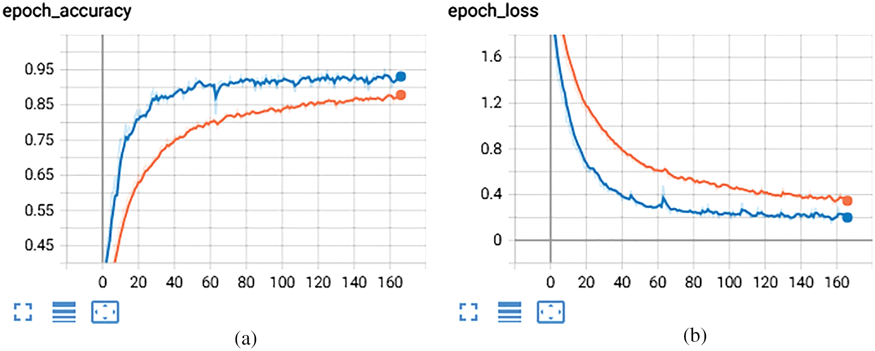
Figure 5: Training and testing accuracy of LSTM (a) LSTM with successive epochs (b) LSTM with successive epochs

4.2 Convolution Neural Network

This model captures patterns in frequency based on sliding windows using Kernel and strides through a convolutional layer. Next, it uses the MaxPooling layer to get the maximum frequency, this process is repeated two times and then a GlobalAveragePooling layer is used to get the average frequency. Later, a Dropout layer is also applied to regularize the model which can prevent overfitting and underfitting, and then the final layer of the model is a Dense layer which uses Softmax as an activation unit to generate the final prediction.

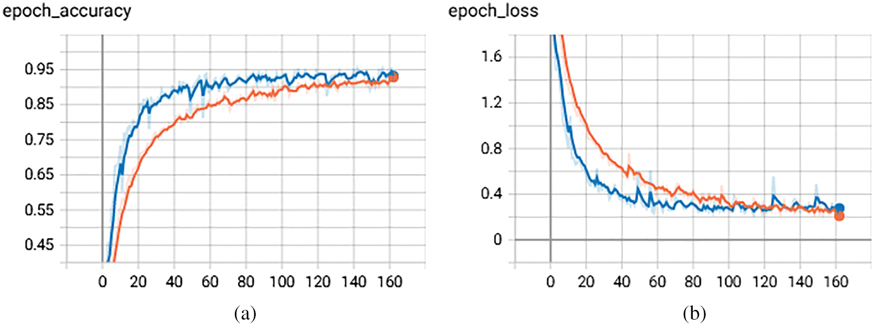
Figure 6: Training and testing accuracy of CNN (a) Accuracy of CNN with successive epochs (b) Loss of CNN with successive epochs

Figs. 6a and 6b discuss the result analysis of training and testing with the loss and accuracy of the CNN model. The result shown in Figs. 6a and 6b depicts that the CNN model shows improvement in terms of accuracy with 95.62% as compared to the previous model (i.e., 93.15%) but in terms of log loss, performance deteriorates with 0.21 as compared to the previous model (i.e., 0.17).

4.3 Combined Approach for LSTM and CNN Analysis

In this model, both CNN and LSTM models are combined. For this, the input layer has been connected to two different layers, one is a Convolutional layer and the other is an LSTM layer. After this, the same layers are used as used in the previous two models. Next, the Dense layer of CNN and LSTM has been combined and a Dropout layer is used to prevent overfitting and underfitting and then the final layer of the model is a Dense layer which uses Softmax as an activation unit to generate the final prediction.

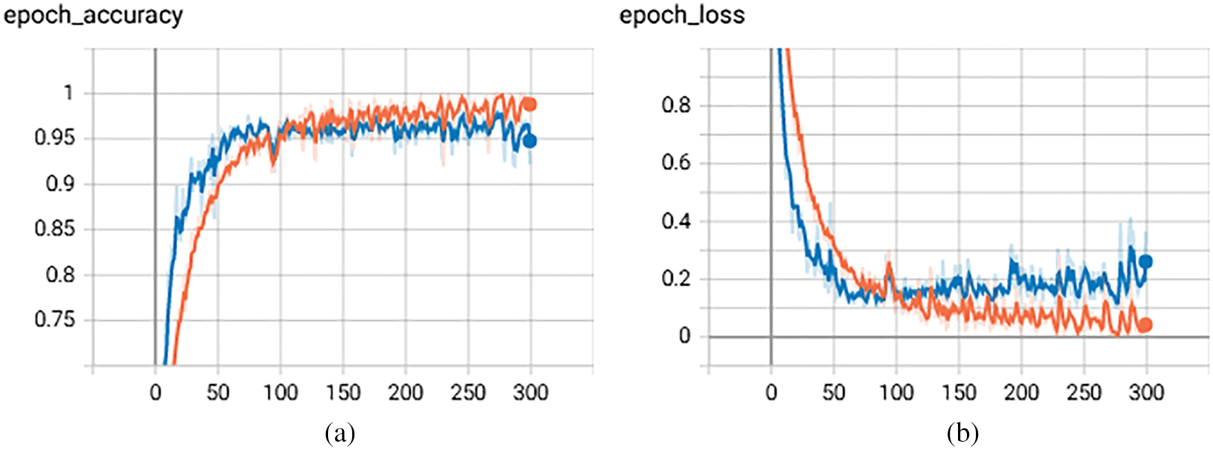
Figure 7: Combination of LSTM and CNN with successive epochs (a) Accuracy of CNN with successive epochs (b) Loss of CNN with successive epochs

Figs. 7a and 7b discuss the result analysis of training and testing with loss and accuracy of the combination of CNN and LSTM model. The result shown in Figs. 7a and 7b depicts that this model performs best with an accuracy of 97.12% and log loss of 0.16.

Receiver Operating Characteristic (ROC) shows how much the model is capable to differentiate between classes. Fig. 8 discusses the result analysis of test data on the ROC curve.

The above-discussed results are shown in Tab. 2 and according to the analysis, CNN performs better based on accuracy and LSTM performs better based on the log loss. Combination of CNN and LSTM performs best in terms of both accuracy and log loss. It also shows the number of parameters for all the models, parameters depend on the number of weights and learned by the model during training.

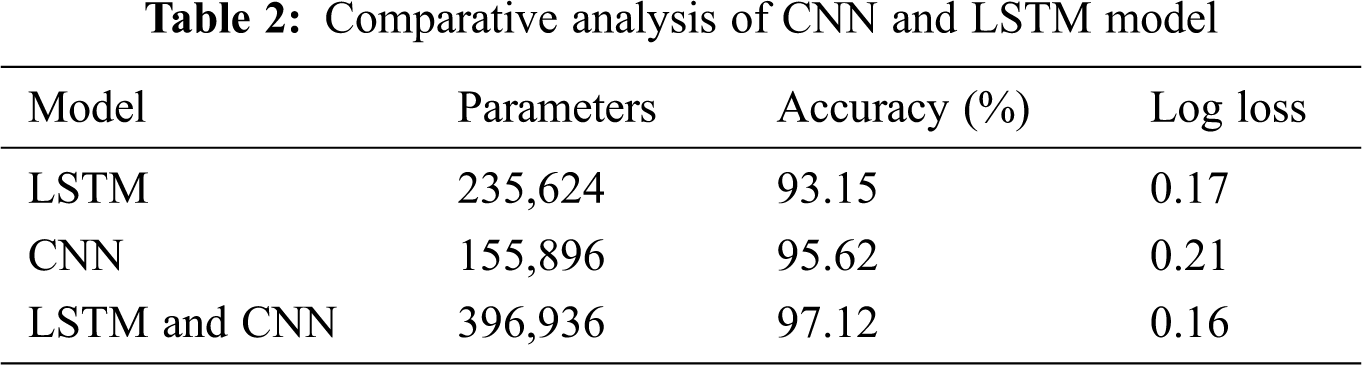
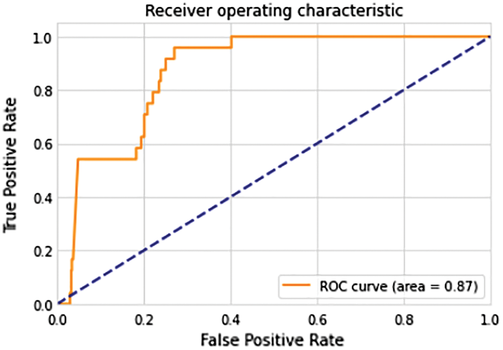
Figure 8: ROC curve for combination of LSTM and CNN

5  Conclusion and Future Scope

Few people show interest these days in becoming a forest ranger. With the scarcity of experts in this area, this paper can be a boon. In this work, multiple models were tried to classify the distinct species of tropical rainforest with the audio signal. The combination of LSTM and CNN showed the best results. The model is created in such a way that it can give almost real-time prediction and does not require high-end GPU to work, making it a lot easier to productionize the model. This work showed particularly superior performance with greater than 97% accuracy and 0.16 multiclass log losses but it can surely be improved with the use of widely popular algorithm like Attention Mechanism. If more data can be collected for more types of species, this model can be retrained so that it can recognize a large variety of species. Also, this model can be deployed in an IoT device.

Funding Statement: The authors received no specific funding for this study.

Conflicts of Interest: The authors declare that they have no conflicts of interest to report regarding the present study.

This work is licensed under a Creative Commons Attribution 4.0 International License, which permits unrestricted use, distribution, and reproduction in any medium, provided the original work is properly cited.