DOI:10.32604/iasc.2022.019887
| Intelligent Automation & Soft Computing DOI:10.32604/iasc.2022.019887 | |
| Article |
Design of Optimal Controllers for Automatic Voltage Regulation Using Archimedes Optimizer
1Department of Electrical Engineering, Faculty of Engineering, Al-Azhar University, Cairo, 11651, Egypt
2Department of Electrical Engineering, Faculty of Engineering, Northern Border University, Arar, 1321, Saudi Arabia
3Department of Electrical Engineering, College of Engineering, Taif University, Taif, 21944, Saudi Arabia
*Corresponding Author: Ahmed Agwa. Email: ah1582009@yahoo.com
Received: 29 April 2021; Accepted: 26 June 2021
Abstract: Automatic voltage regulators (AVRs) in electrical grids preserve the voltage at its nominal value. Regulating the parameters of proportional–integral–derivative (PID) controllers used for AVRs is a nonlinear optimization issue. The objective function is designed to minimize the settling time, rise time, and overshoot of step response of resultant voltage with subjugation to constraints of PID controller parameters. In this study, we suggest using an Archimedes optimization algorithm (AOA) to tune the parameters of the PID controllers for AVRs. In addition, using an AOA to optimize the parameters of a fractional-order PID (FOPID) controller and a PID plus second-order derivative (PIDD2) controller for AVRs is also investigated to validate their effectiveness. The disturbance repudiation and robustness of the AOA-PID controllers are also examined and confirmed. To validate the results of the AOA-PID controllers, they are compared with those of other optimized controllers for convergence speed, the quality of the step response. The results indicate that the AOA functions perfectly and it has good potential for optimizing the PID controller parameters with better step response compared with the PID controller based on other approaches while preferring the results of the AOA–PIDD2 controller over other kinds of the AOA-PID controllers.
Keywords: Automatic voltage regulator; PID controller; parameter tuning; optimization methods; Archimedes optimizer
An electrical power grid is a complex system with many electrical components that are responsible for electric power generation, transmission, and distribution. In power networks, maintaining the stability and constancy of the voltage level is a major problem. If the voltage is different from its rated level, the performance of this equipment will be deteriorated. Another reason for achieving this control is that the real losses in the transmission system depend on both active and reactive power flow [1–3].
The excitation system is an important part of the synchronous generator, which acts as the most widespread control system to maintain the voltage level among numerous voltage-regulation devices. However, the essential part of the excitation system is called the automatic voltage regulator (AVR), which is responsible for adjusting the voltage level at the terminals of the synchronous generators under different operating conditions [4]. Also, it is implemented in the power system network to control the reactive power flow as well as guarantee appropriate participation of the reactive power among the synchronous generators that are connected in parallel. So, the constancy of the AVR system against the varying exciter voltage affects the power system security [5].
The refinement of AVR performance is very important, because of the difficulties in achieving the stability and fast response of AVR due to the load variations and high inductance field windings of the alternator [6,7].
This study deals with the control and the operating system of the AVR. The proportional–integral–derivative (PID) is the most used controller of AVR systems due to its robust performance under different operating conditions as well as the simplicity of structure [8–11]. The standard PID (SPID) controller encompasses three control parameters: the proportional gain (Kp), the integral gain (Ki), and the derivative gain (Kd) [12–16].
Furthermore, few studies used the real PID (RPID) controller presented in [17–20] in which the derived action was filtered, so the RPID controller adds another parameter called the filter coefficient N to the three conventional parameters. There is also other modification over the PID controller namely PID with the derivative of second order (PIDD2) as developed in [21,22] where PIDD2 controller involving four parameters namely Kp, Ki, Kd, and Kd2, where Kd2 is the gain of second-order derivative. Moreover, the fractional order PID controller (FOPID) was developed by adding the fractional calculus to the PID controller as introduced in [23–28] to improve the performance of the PID controller. The FOPID controller includes five parameters, viz. Kp, Ki, Kd, λ, and µ, where λ and µ define the order of integration and differentiation, respectively [29,30].
To provide the desirable voltage response of the AVR system, the optimal parameters of the controllers should be tuned, and, for this purpose, numerous heuristic optimization techniques, such as the genetic algorithm [25,27,31,32], differential evolution [33], particle swarm optimization (PSO) algorithm [14,23], local unimodal sampling algorithm [34], teaching learning-based optimization (TLBO) algorithm [18,35], ant colony optimization (ACO) [19,36], artificial bee colony algorithm [37], cuckoo search (CS) algorithm [20,28], chaotic ant swarm (CAS) algorithm [38], symbiotic organisms search [9], multi-objective extremal optimization [26], harmony search algorithm [35], whale optimization algorithm [21,39], and manta ray foraging optimizer (MRFO) [40], have been used.
Despite this brief literature survey, the no-free-launch theorem guides us that the estimation of the controller parameters is likely improved based on the recent optimization techniques. So, in this study, a new algorithm called Archimedes optimization algorithm (AOA) that has been presented in 2021 [41], is implemented to identify the optimal parameters of SPID, RPID, FOPID, and PIDD2 controllers to establish their optimal setting. Also, to achieve this goal, the construction of AVR that was presented in the literature is used. The AOA is inspired using the Archimedes’ principle that describes the forces acting on an object immersed in a fluid. The AOA is chosen because its published results are hopeful and outperform other optimizers. Utilization of the AOA has succeeded for optimum distributed generations [42,43].
Performance assessments are carried out to confirm the effectiveness of applying the AOA-based technique. However, all controllers tuned by the AOA are compared with other controllers that are optimized by other reported techniques for convergence speed and quality of step response to validate the superiority of the AOA-PID controllers. The superiority of the AOA-PID controllers is validated by comparing their convergence speed, their quality of step response with other controllers that are optimized by other reported techniques. The disturbance repudiation and the robustness of the AOA-PID controllers are analyzed and proved. In addition, to decide which is the most suitable controller as a regulator in the AVR systems, a comparative study is also carried out. The main contribution of this study is described as follows:
• Innovative use of the AOA for identification of the controller parameters.
• Four types of controllers (SPID, RPID, FOPID, and PIDD2) are examined and analyzed for defining the most suitable controller.
• Comparison of the AOA-PID controllers with other controllers that are tuned by recent optimizers based on simulation results.
• Investigating the robustness of the AOA based on the controlled AVR system during parametric variation of the system model.
The paper is organized as follows: In Section 2, the modeling of the AVR system and the structure of four different kinds of PID controllers are introduced. The objective function is mathematically formulated in Section 4. Section 4 presents a short overview of the AOA. Section 5 presents the simulation results obtained using the AOA-PID controllers for the AVR and other compared techniques as well as discussion. Section 6 concludes this paper.
Disturbances are the commonly found phenomena in electrical systems, which in turn lead to voltage fluctuations and oscillations. These voltage variations deteriorate the equipments in the power system. The AVR is used in these electrical systems to maintain their voltage level at a prescribed value by correcting their terminal voltage. It is installed at many places in the power system, such as generators, transformers, and feeders.
Fig. 1 shows the main components of the AVR used to control the terminal voltage of a generator. The main parts of the AVR are controllers, amplifiers, exciters, and sensors. The plant voltage VP(s) is measured and compared with a prescribed value Vref(s) and the error signal V(s) is sent to the controller to calculate the required control signal U(s) that is amplified through the amplifier. The amplifier error signal is used to control the exciter of the generator, which in turn controls the generator terminal voltage VP(s).

Figure 1: AVR block diagram
The transfer functions of all AVR components, except the controller, are first order with dimensionless gain (K) and time constant (T). The utilized AVR in the literature has nominal values of gains and time constants of amplifier, exciter, generator, and sensor as follows: KA = 10, KE = 1, KG = 1, KS = 1, TA = 0.1, TE = 0.4, TG = 1, and TS = 0.01, respectively [18–22]. The aforesaid values of gains and time constants are used in this study to validate the comparison with previous approaches.
The controller is the pivotal VAR component that is used to improve the system dynamic performance. The PID controller is one of the well-known controllers with four kinds, viz. the SPID, the RPID, the FOPID, and the PIDD2 whose transfer functions are given in (1)−(4), respectively [40]. Generally, the SPID controller possesses tuning three parameters Kp, Ki, and Kd. There are additional parameters for other kinds of PID controllers as follows: N for the RPID controller, λ and µ for the FOPID controller, and Kd2 for the PIDD2 controller.
3 Objective Function Formulation
Generally, the parameters of the PID controller to be optimized are either 3–5, depending on its kind. The researchers used numerous objective functions for tuning the parameters of the SPID, RPID, and FOPID controllers, but we have found in the literature that using the following objective function (OF1) yields the best results when compared with others since it guarantees the equilibrium among speed, overshoot, and steady-state error, so it is employed in this research.
where β is a constant whose value is 1, OV is the overshoot (%), Ess symbolizes the steady-state error (pu), ts is the settling time (s), and tr is the rise time (s).
Tuning the parameters of the PIDD2 controller using OF1 does not give the best results since its different construction due to the inclusion of additional second-order derivative, thus different objective function (OF2) is innovatively suggested to tune its parameters.
where w1−w5 are the weighting factors, whose values are 6, 4, 2, 1, and 1, respectively, and e is the error signal.
Both OF1 and OF2 are subjugated to constraints which are defined by the upper and lower limits of the PID controller parameters.
Lately, introduced metaheuristic techniques, especially those inspired using physics, have created an interesting result. AOA was inventive with inspirations based on the Archimedes’ principle. It mimics the principle of buoyancy force that exerted upward on the object, completely or partially submerged in a fluid and is proportional to the weight of the fluid that has been displaced. However, when the weight of the object is greater than the weight of the fluid displaced, the object will sink. In contrast, the object will float when the object’s weight is equal to the weight of the fluid displaced. In AOA, the objects submerged in the fluid are considered as the population individuals. These objects have volume, acceleration, and density which have a major impact on the buoyancy of the object. The concept of AOA is based on reaching the point at which the objects are neutrally buoyant, where the fluid force is equal to zero.
AOA ensures a notable balance between exploitation and exploration that makes AOA appropriate for solving the complex optimization problems that consist of many local solutions since it stores solutions population and investigates a wide extent to find the best optimal global solution.
Furthermore, AOA has a simple design with only a few control parameters; still it is powerful and robust as proved in [41]. In addition, it has the ability to adjust the candidate solutions pool to avoid the trap or located at the suboptimal locations.
Similar to other metaheuristic algorithms based on population, AOA also starts the searching process through initial objects (population) as a candidate solution with random densities, volumes, and accelerations. At this step, all objects are also initialized with their random positions in the fluid. After evaluation of the initial population fitness, AOA works in iterations until it meets the conditions. During each iteration, AOA updates the volume and density of each object. Then, based on the condition of its collision with other adjacent objects, the acceleration of each object is updated. The updated volume, density, and acceleration compute the new position of each object [42]. The mathematical formulation of AOA is described as follows.
The position of each object is initialized as follows:
where xk is the k-numbered object, N is the population, and llk and ulk are the lower and upper limits of the search space, respectively. Volume (Volk), density (Denk), and acceleration (Acck) for each object are initialized as below:
where
4.2 Update of the Volumes and Densities
The volume and density of the k-numbered object for the iteration t + 1 is updated as follows:
where Denbest and Volbest are the density and volume of the best-found object and rand is a random number that is uniformly distributed.
4.3 Transfer Factor and Density Operator
Initially, a collision occurs between objects and after some time, the objects endeavor to reach the equilibrium state. This is carried out in AOA by transfer factor TF that is used to transform the search from exploration to exploitation. It also increases progressively with time till reaching 1 and is described as below:
where t and tmax are the iteration number and the maximum number of iterations, respectively. Similarly, the density decreasing operator D helps AOA in global search.
where Dt + 1 decreases with time, providing the ability to converge to the identified promising region. It is worth noting that proper treatment of this variable will guarantee the balance between exploitation and exploration within AOA.
4.4.1 The Existence of Collision Among Objects
The occurrence of collision among objects takes place at TF ≤ 0.5 [43]. After selecting the random material (rm), for iteration t + 1, the object's acceleration
where Volrm, Denrm, and Accrm are the volume, density, and acceleration of rm, respectively.
4.4.2 The Absence of Collision Among Objects
The collision among objects is blocked at TF > 0.5. Therefore, the object’s acceleration is updated at iteration t + 1 as stated in the following equation:
where Accbest is the acceleration of the best object.
4.4.3 Normalization of Acceleration
To calculate the percentage of change, the acceleration of the object is normalized as below:
where L and U are the normalization range and set to 0.1 and 0.9, respectively.
However,
The used equations include four constants C1–C4 and their values in engineering problems are 2, 6, 2, 0.5, respectively [41]. For iteration t + 1, the exploration stage (if TF ≤ 0.5), the position of k-numbered object
where
Furthermore, at the exploitation stage (TF > 0.5), the positions of objects are updated as below:
where T is proportional to TF and increases with time and it is described as
Also, F is the flag for changing the motion direction according to the following equation:
Each object is evaluated using the OF and the best solution is remembered, that is, xbest, Volbest, Denbest, and Accbest are assigned.
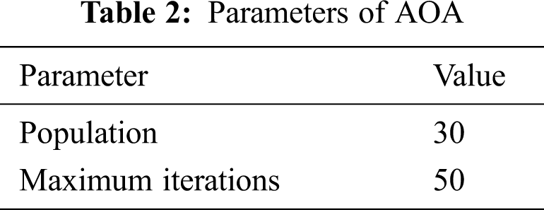
This section includes the obtained results of applying AOA to optimize the parameters of four kinds of the PID controller for AVR, namely SPID, RPID, FOPID, and PIDD2. Tab. 1 presents the upper and lower bounds for the parameters of the four kinds of the PID controller. Tab. 2 lists the parameters of AOA. All four kinds of the AOA-PID controller are compared with other optimizers, according to their results.

The increase in reference voltage from 0 to 1 pu at t = 0 is simulated to examine the performance of the SPID, RPID, FOPID, and PIDD2 controllers for AVR. Tab. 3 lists the optimized gains of the four kinds of the PID controller for AVR using AOA.

The convergence curve of the AOA-PIDD2 controller with other kinds of the AOA-PID controller for AVR is displayed in Fig. 2a for comparison, and it is also displayed in Fig. 2b because its OF2 is different. In general, the AOA-PIDD2 controller attains the best convergence in terms of the minimum OF and convergence speed.
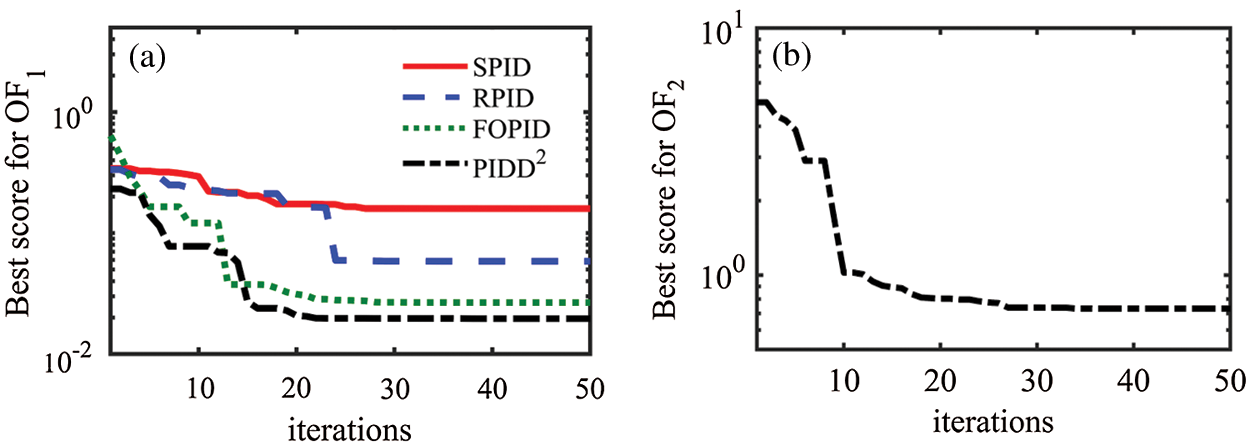
Figure 2: The OF convergence curves of the PID controllers using AOA: (a) AOA-PID controller; (b) AOA-PIDD2 controller
The performance of AOA in optimizing the PID controllers for AVR is validated by comparing with other approaches in the literature according to the time-domain analysis of step response in terms of ts, tr, and OV, as summarized in Tab. 4. We can see that both the AOA-SPID and AOA-RPID controllers result in smaller ts and tr, that is, faster response than the corresponding controllers which were optimized by other approaches via the same OF1 in the literature, with maintaining the OV at the acceptable values.
The value of ts produced by the AOA-FOPID controller is the smallest in comparison with other tuned FOPID controllers regardless of tr of the AOA-FOPID controller being slightly higher than that of the CS-FOPID controller in [28] due to the obvious smallness of ts of the AOA-FOPID controller. The OV obtained using the AOA-FOPID controller is preserved at satisfactory values. Therefore, we can declare that the AOA-SPID, AOA-RPID, and AOA-FOPID controllers yield a better step response than the corresponding controllers based on other optimizers.

Furthermore, Tab. 4 also shows that the AOA-PIDD2 controller produces a faster response than both the WOA-PIDD2 controller in [21] and the PSO-PIDD2 controller in [22], with maintaining the OV at the satisfactory values. The AOA-PIDD2 controller results in lesser OV than the MRFO-PIDD2 controller in [40] with almost the same ts and tr, that is, the response speed is approximately equal. Consequently, we can say that the AOA-PIDD2 controller attains better equilibrium among speed and overshoot than other optimized PIDD2 controllers. The following OFs are in [21,22,40] for the optimizers of the PIDD2 controller with which the AOA-PIDD2 controller is compared:
Fig. 3 shows the resultant voltage of AVR, which is controlled by the AOA-PID controllers. It reveals that the kinds of the PID controller can be arranged according to the response speed and overshoot as following the PIDD2 controller, FOPID controller, SPID controller, and then RPID controller, and Tab. 4 details this arrangement using a quantitative performance assessment.
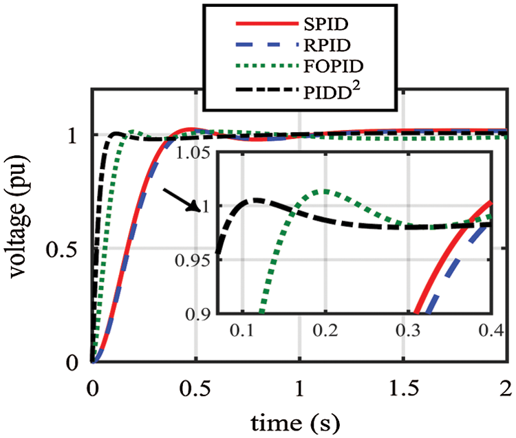
Figure 3: Resultant voltage of step response using various AOA-PID controllers
The time constants of the amplifier, exciter, generator, and sensor are changed from −50% to +50% of their nominal values to analyze the performance robustness of the AOA-PID controllers for AVR. The resultant voltages of step response during variations of the time constants are revealed in Figs. 4−7, where the AOA-PID controllers exhibit robustness against inconstancy of the time constants.
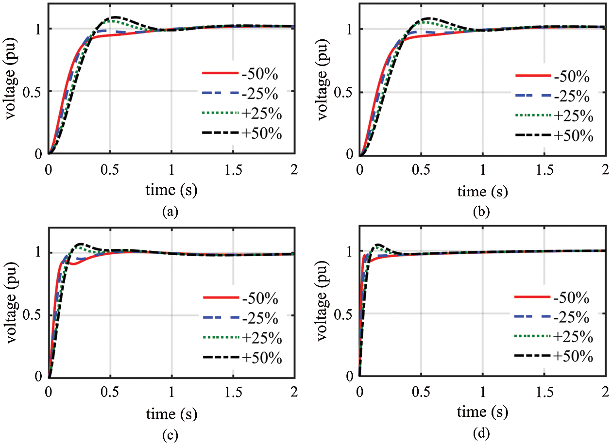
Figure 4: Resultant voltage of step response throughout changing TA from −50% to +50% of the nominal value: (a) SPID controller; (b) RPID controller; (c) FOPID controller; (d) PPID2 controller
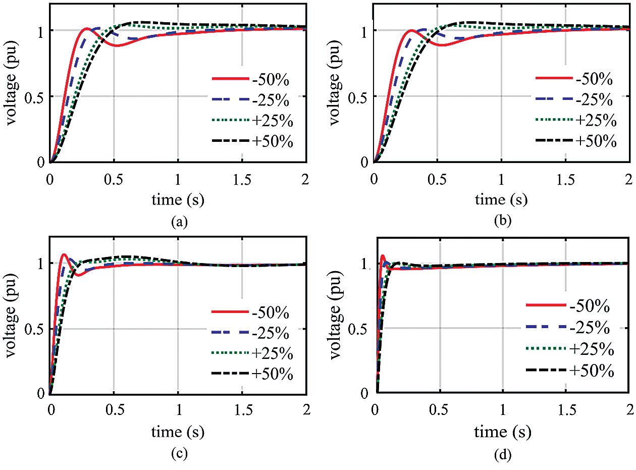
Figure 5: Resultant voltage of step response throughout changing TE from −50% to +50% of the nominal value: (a) SPID controller; (b) RPID controller; (c) FOPID controller; (d) PPID2 controller
Tab. 5 lists the time-domain analysis of step response throughout changing the time constants where the values of tr, ts, and OV do not significantly differ from those under nominal status. We can observe that PIDD2 controller is the least affected by variations in the time constants; conversely, the SPID and RPID controllers are the most affected. We also notice that changing the time constant of the generator significantly affects the resultant voltage, whereas changing the time constant of the sensor has the least effect on the resultant voltage.

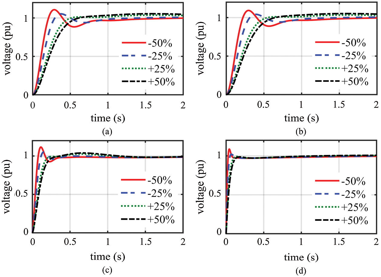
Figure 6: Resultant voltage of step response throughout changing TG from −50% to +50% of the nominal value: (a) SPID controller; (b) RPID controller; (c) FOPID controller; (d) PPID2 controller
5.3 Analysis of Disturbance Rejection
The capability of the AOA-PID controllers for AVR to reject disturbances is analyzed by testing the subjection to both the disturbed control signal and the disturbed load, as shown in Fig. 8.
The disturbed output of the controller is simulated as a step signal of 1 pu in the interval starting at t = 2 s and ending at t = 8 s. In addition, the disturbed load is also simulated as a step signal of 0.3 pu in the interval starting at t = 2 s and ending at t = 3.5 s. The disturbances and the corresponding resultant voltages are displayed in Figs. 9−12, which reveals the AOA-PID controllers’ capability of disturbances rejection since they quickly stabilize the voltage at its nominal value. We can see that the PIDD2 controller has the best capability of stabilizing voltage in terms of speed and overshoot.
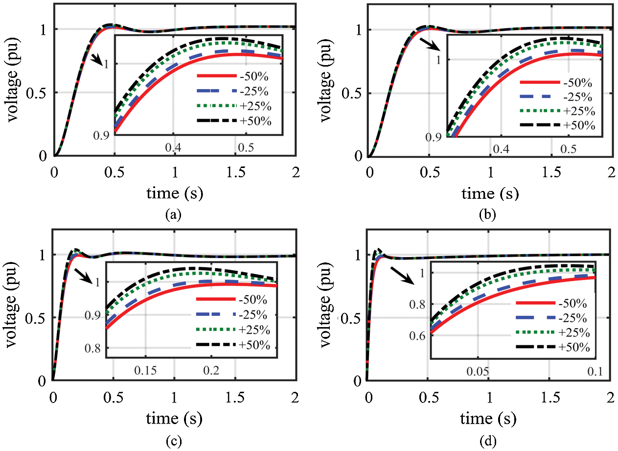
Figure 7: Resultant voltage of step response throughout changing TS from −50% to +50% of the nominal value: (a) SPID controller; (b) RPID controller; (c) FOPID controller; (d) PPID2 controller
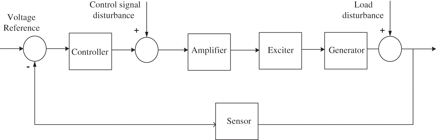
Figure 8: AVR block diagram with disturbances
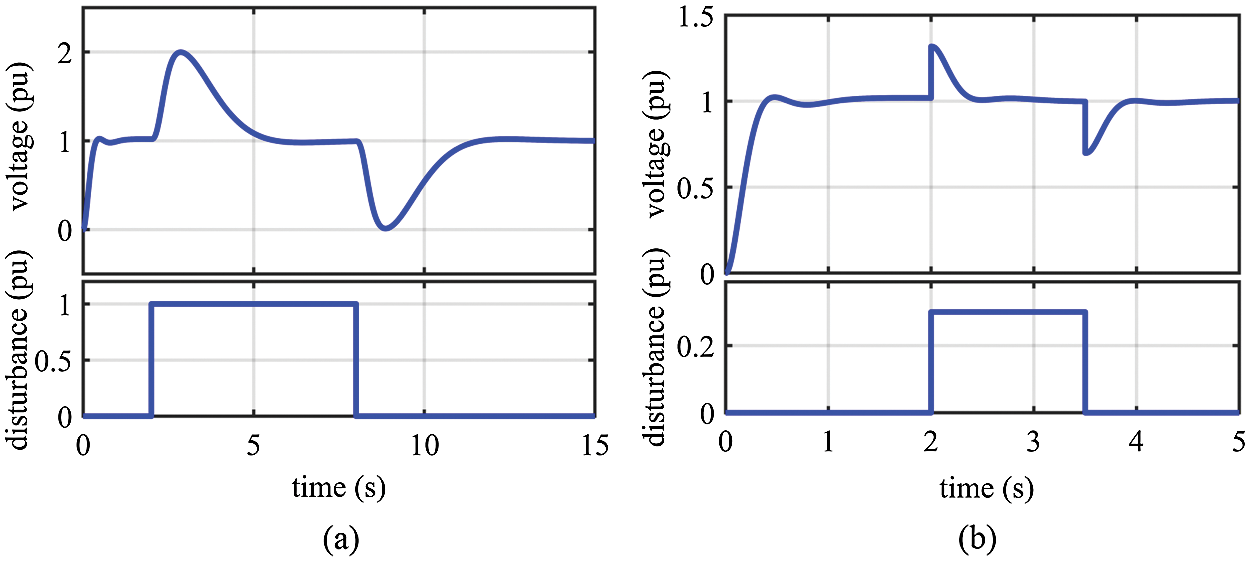
Figure 9: Resultant voltage of step response for the AOA-SPID controller under disturbances: (a) under disturbed control signal; (b) under disturbed load
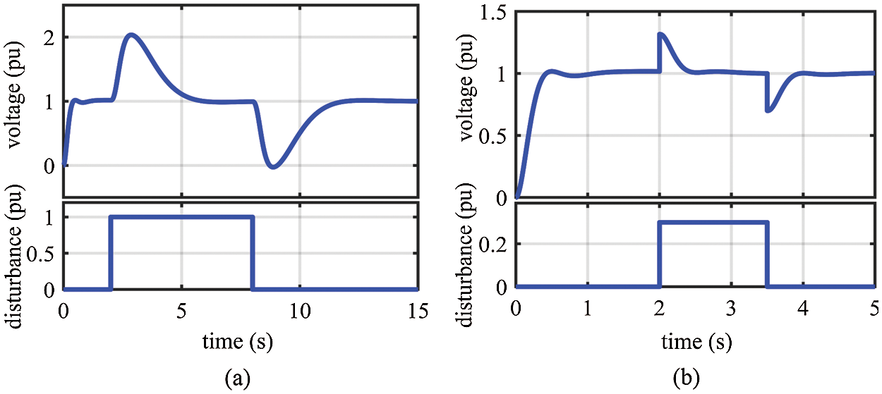
Figure 10: Resultant voltage of step response for the AOA-RPID controller under disturbances: (a) under disturbed control signal; (b) under disturbed load
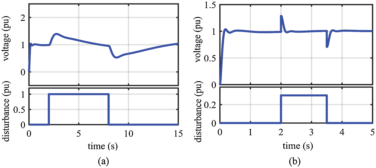
Figure 11: Resultant voltage of step response for the AOA-FOPID controller under disturbances: (a) under disturbed control signal; (b) under disturbed load
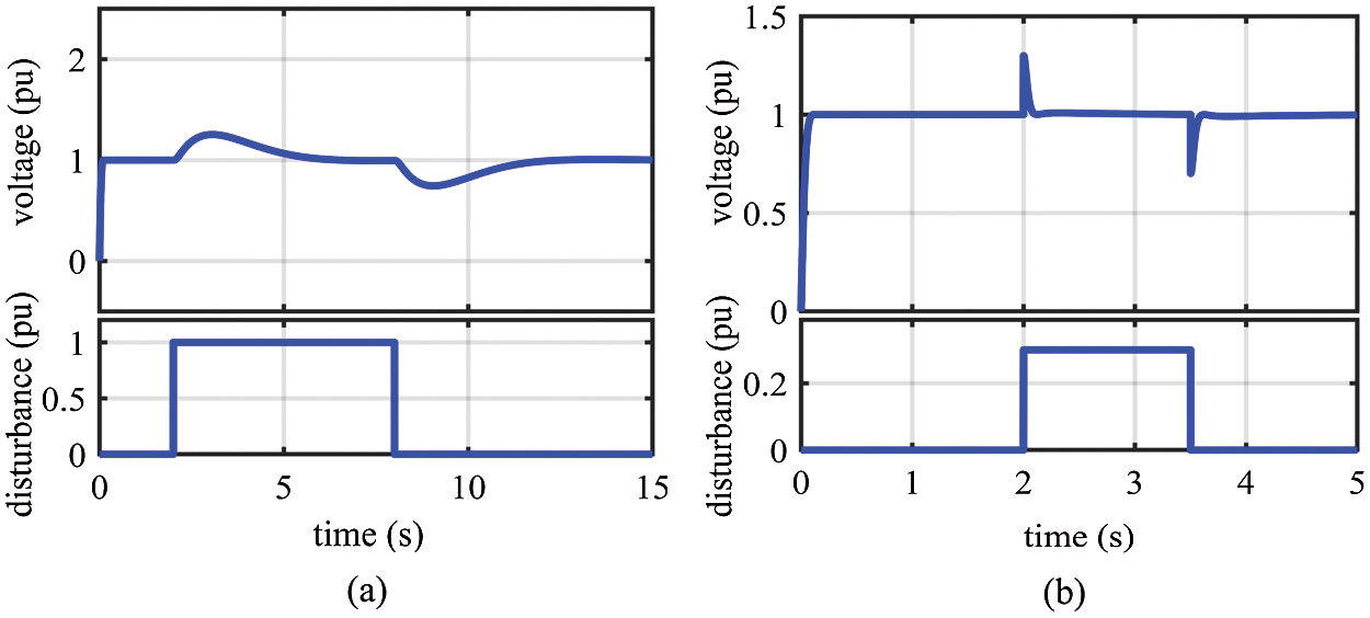
Figure 12: Resultant voltage of step response for the AOA-PIDD2 controller under disturbances: (a) under disturbed control signal; (b) under disturbed load
In electrical networks, AVR is used to maintain the voltage at a prescribed value. We have used AOA for optimizing the parameters of the PID controllers for AVR. In addition, the AOA-FOPID controller and the AOA-PIDD2 controller for AVR are also used. The objective function minimizes the settling time, rise time, and overshoot of step response of voltage with restriction of the PID controller parameters within the predefined limits. The results of the AOA-PID controllers for AVR are compared with those of the other algorithms, which indicate that AVRs with the AOA-PID controllers result in the best step response since they achieve better balance among speed and overshoot. The work of the AOA-PID controllers for AVR during abnormal status, for example, variations in time constants and disturbances, has been proved to be perfect in the simulation results. In addition, comparisons among the kinds of AOA-PID controllers revealed that the AOA-PIDD2 controller has the best performance.
Acknowledgement: The authors gratefully acknowledge the approval and the support of this research study by Taif University Researchers Supporting Project Number (TURSP-2020/146), Taif University, Taif, Saudi Arabia.
Funding Statement: This work was supported by Taif University Researchers Supporting Project Number (TURSP-2020/146), Taif University, Taif, Saudi Arabia.
Conflicts of Interest: The authors declare that they have no conflicts of interest to report regarding the present study.
1. A. I. Omar, S. H. Abdel-Aleem, E. E. El-Zahab, M. Algablawy and Z. M. Ali, “An improved approach for robust control of dynamic voltage restorer and power quality enhancement using grasshopper optimization algorithm,” ISA Transactions, vol. 95, pp. 110–129, 2019. [Google Scholar]
2. A. Sikander and P. Thakur, “A new control design strategy for automatic voltage regulator in power system,” ISA Transactions, vol. 100, no. 2B, pp. 235–243, 2020. [Google Scholar]
3. H. Gozde, “Robust 2DOF state-feedback PI-controller based on meta-heuristic optimization for automatic voltage regulation system,” ISA Transactions, vol. 98, no. Issue 4, pp. 26–36, 2020. [Google Scholar]
4. S. Essallah, A. Bouallegue and A. Khedher, “AVR and PSS controller integration in a power system: Small-signal stability study with DFIG,” IEEE/CAA Journal of Automatica Sinica, vol. 1, no. 1, pp. 55–65, 2018. [Google Scholar]
5. I. Boldea, Synchronous Generators, 2nd ed., Boca Raton, FL, USA: CRC Press, pp. 270–283, 2016. [Google Scholar]
6. P. Kundur, Power System Stability and Control, 1st ed., NY, USA: McGraw-Hill, pp. 987–995, 1994. [Google Scholar]
7. K. H. Ang, G. Chong and Y. Li, “PID control system analysis, design, and technology,” IEEE Transactions on Control Systems Technology, vol. 13, no. 4, pp. 559–576, 2005. [Google Scholar]
8. S. Ekinci and B. Hekimoğlu, “Improved kidney-inspired algorithm approach for tuning of PID controller in AVR system,” IEEE Access, vol. 7, pp. 39935–39947, 2019. [Google Scholar]
9. E. Çelik and R. Durgut, “Performance enhancement of automatic voltage regulator by modified cost function and symbiotic organisms search algorithm,” Engineering Science and Technology, An International Journal, vol. 21, no. 5, pp. 1104–1111, 2018. [Google Scholar]
10. S. Panda, B. K. Sahu and P. K. Mohanty, “Design and performance analysis of PID controller for an automatic voltage regulator system using simplified particle swarm optimization,” Journal of the Franklin Institute, vol. 349, no. 8, pp. 2609–2625, 2012. [Google Scholar]
11. D. H. Kim, “Hybrid GA-BF based intelligent PID controller tuning for AVR system,” Applied Soft Computing, vol. 11, no. 1, pp. 11–22, 2011. [Google Scholar]
12. H. Gozde and M. C. Taplamacioglu, “Comparative performance analysis of artificial bee colony algorithm for automatic voltage regulator (AVR) system,” Journal of the Franklin Institute, vol. 348, no. 8, pp. 1927–1946, 2011. [Google Scholar]
13. L. S. Coelho, “Tuning of PID controller for an automatic regulator voltage system using chaotic optimization approach,” Chaos, Solitons & Fractals, vol. 39, no. 4, pp. 1504–1514, 2009. [Google Scholar]
14. Z. Gaing, “A particle swarm optimization approach for optimum design of PID controller in AVR system,” IEEE Transactions on Energy Conversion, vol. 19, no. 2, pp. 384–391, 2004. [Google Scholar]
15. A. Chatterjee, V. Mukherjee and S. P. Ghoshal, “Velocity relaxed and craziness-based swarm optimized intelligent PID and PSS controlled AVR system,” International Journal of Electrical Power & Energy Systems, vol. 31, no. 7–8, pp. 323–333, 2009. [Google Scholar]
16. H. Zhu, L. Li, Y. Zhao, Y. Guo and Y. Yang, “CAS algorithm-based optimum design of PID controller in AVR system,” Chaos, Solitons & Fractals, vol. 42, no. 2, pp. 792–800, 2009. [Google Scholar]
17. M. A. Sahib and B. S. Ahmed, “A new multiobjective performance criterion used in PID tuning optimization algorithms,” Journal of Advanced Research, vol. 7, no. 1, pp. 125–134, 2016. [Google Scholar]
18. S. Chatterjee and V. Mukherjee, “PID controller for automatic voltage regulator using teaching-learning based optimization technique,” International Journal of Electrical Power & Energy Systems, vol. 77, no. 4, pp. 418–429, 2016. [Google Scholar]
19. M. Blondin, P. Sicard and P. M. Pardalos, “Controller tuning approach with robustness, stability and dynamic criteria for the original AVR System,” Mathematics and Computers in Simulation, vol. 163, no. 7, pp. 168–182, 2019. [Google Scholar]
20. Z. Bingul and O. Karahan, “A novel performance criterion approach to optimum design of PID controller using cuckoo search algorithm for AVR system,” Journal of the Franklin Institute, vol. 355, no. 13, pp. 5534–5559, 2018. [Google Scholar]
21. D. Mokeddem and S. Mirjalili, “Improved whale optimization algorithm applied to design PID plus second-order derivative controller for automatic voltage regulator system,” Journal of the Chinese Institute of Engineers, vol. 43, no. 6, pp. 541–552, 2020. [Google Scholar]
22. M. A. Sahib, “A novel optimal PID plus second order derivative controller for AVR system,” Engineering Science and Technology, an International Journal, vol. 18, no. 2, pp. 194–206, 2015. [Google Scholar]
23. M. Zamani, M. Karimi-Ghartemani, N. Sadati and M. Parniani, “Design of a fractional order PID controller for an AVR using particle swarm optimization,” Control Engineering Practice, vol. 17, no. 12, pp. 1380–1387, 2009. [Google Scholar]
24. I. Pan and S. Das, “Chaotic multi-objective optimization based design of fractional order PIλDμ controller in AVR system,” International Journal of Electrical Power & Energy Systems, vol. 43, no. 1, pp. 393–407, 2012. [Google Scholar]
25. I. Pan and S. Das, “Frequency domain design of fractional order PID controller for AVR system using chaotic multi-objective optimization,” International Journal of Electrical Power & Energy Systems, vol. 51, pp. 106–118, 2013. [Google Scholar]
26. G. Zeng, J. Chen, Y. Dai, L. Li, C. Zheng et al., “Design of fractional order PID controller for automatic regulator voltage system based on multi-objective extremal optimization,” Neurocomputing, vol. 160, pp. 173–184, 2015. [Google Scholar]
27. M. E. Ortiz-Quisbert, M. A. Duarte-Mermoud, F. Milla, R. Castro-Linares and G. Lefranc, “Optimal fractional order adaptive controllers for AVR applications,” Electrical Engineering, vol. 100, pp. 267–283, 2018. [Google Scholar]
28. A. Sikander, P. Thakur, R. C. Bansal and S. Rajasekar, “A novel technique to design cuckoo search based FOPID controller for AVR in power systems,” Computers and Electrical Engineering, vol. 70, no. 1, pp. 261–274, 2018. [Google Scholar]
29. J. Viola, L. Angel and J. M. Sebastian, “Design and robust performance evaluation of a fractional order PID controller applied to a DC motor,” IEEE/CAA Journal of Automatica Sinica, vol. 4, no. 2, pp. 304–314, 2017. [Google Scholar]
30. A. S. Chopade, S. W. Khubalkar, A. S. Junghare, M. V. Aware and S. Das, “Design and implementation of digital fractional order PID controller using optimal pole-zero approximation method for magnetic levitation system,” IEEE/CAA Journal of Automatica Sinica, vol. 5, no. 5, pp. 977–989, 2018. [Google Scholar]
31. H. M. Hasanien, “Design optimization of PID controller in automatic voltage regulator system using Taguchi combined genetic algorithm method,” IEEE Systems Journal, vol. 7, no. 4, pp. 825–831, 2012. [Google Scholar]
32. J. Ye, “PID tuning method using single-valued neutrosophic cosine measure and genetic algorithm,” Intelligent Automation & Soft Computing, vol. 25, no. 1, pp. 15–23, 2019. [Google Scholar]
33. T. Chen and M. Yeh, “Optimized PID controller using adaptive differential evolution with mean of p-best mutation strategy,” Intelligent Automation & Soft Computing, vol. 26, no. 3, pp. 407–420, 2020. [Google Scholar]
34. P. K. Mohanty, B. K. Sahu and S. Panda, “Tuning and assessment of proportional-integral–derivative controller for an automatic voltage regulator system employing local unimodal sampling algorithm,” Electric Power Components and Systems, vol. 42, no. 9, pp. 959–969, 2014. [Google Scholar]
35. A. M. Mosaad, M. A. Attia and A. Y. Abdelaziz, “Comparative performance analysis of AVR controllers using modern optimization techniques,” Electric Power Components and Systems, vol. 46, no. 19–20, pp. 2117–2130, 2018. [Google Scholar]
36. M. Blondin, J. Sanchis, P. Sicard and J. M. Herrero, “New optimal controller tuning method for an AVR system using a simplified ant colony optimization with a new constrained Nelder–Mead algorithm,” Applied Soft Computing, vol. 62, no. 6, pp. 216–229, 2018. [Google Scholar]
37. D. Zhang, T. Ying-Gan and G. Xin-Ping, “Optimum design of fractional order PID controller for an AVR system using an improved artificial bee colony algorithm,” Acta Automatica Sinica, vol. 40, no. 5, pp. 973–979, 2014. [Google Scholar]
38. Y. Tang, M. Cui, C. Hua, L. Li and Y. Yang, “Optimum design of fractional order PIλDμ controller for AVR system using chaotic ant swarm,” Expert Systems with Applications, vol. 39, no. 8, pp. 6887–6896, 2012. [Google Scholar]
39. A. M. Mosaad, M. A. Attia and A. Y. Abdelaziz, “Whale optimization algorithm to tune PID and PIDA controllers on AVR system,” Ain Shams Engineering Journal, vol. 10, no. 4, pp. 755–767, 2019. [Google Scholar]
40. M. Micev, M. Ćalasan, Z. M. Ali, H. M. Hasanien and S. H. Abdel-Aleem, “Optimal design of automatic voltage regulation controller using hybrid simulated annealing-Manta ray foraging optimization algorithm,” Ain Shams Engineering Journal, vol. 12, no. 1, pp. 641–657, 2021. [Google Scholar]
41. F. A. Hashim, K. Hussain, E. H. Houssein, M. S. Mabrouk and W. Al-Atabany, “Archimedes optimization algorithm: A new metaheuristic algorithm for solving optimization problems,” Applied Intelligence, vol. 51, no. 3, pp. 1–21, 2021. [Google Scholar]
42. Z. M. Ali, I. M. Diaaeldin, A. El-Rafei, H. M. Hasanien, S. A. Abdel-Aleem et al., “A novel distributed generation planning algorithm via graphically-based network reconfiguration and soft open points placement using Archimedes optimization algorithm,” Ain Shams Engineering Journal, (in press2021. [Google Scholar]
43. Y. Li, H. Zhu, D. Wang, K. Wang, W. Kong et al., “Comprehensive optimization of distributed generation considering network reconstruction based on Archimedes optimization algorithm,” in Proc. IOP Conf. Series: Earth and Environmental Science, Chongqing, China, 2021. [Google Scholar]
 | This work is licensed under a Creative Commons Attribution 4.0 International License, which permits unrestricted use, distribution, and reproduction in any medium, provided the original work is properly cited. |