Intelligent Automation & Soft Computing DOI:10.32604/iasc.2022.020127
Article

An Optimal Anchor Placement Method for Localization in Large-Scale Wireless Sensor Networks

Tuğrul Çavdar1, Faruk Baturalp Günay2,*, Nader Ebrahimpour1 and Muhammet Talha Kakız3

1Department of Computer Engineering, Karadeniz Technical University, Trabzon, 61080, Turkey
2Department of Computer Engineering, Faculty of Engineering, Atatürk University, Erzurum, 25050, Turkey
3Department of Computer Engineering, Faculty of Engineering, Osmaniye Korkut Ata University, Osmaniye, 80000, Turkey
*Corresponding Author: Faruk Baturalp Günay. Email: baturalp@atauni.edu.tr
Received: 10 May 2021; Accepted: 21 June 2021

Abstract: Localization is an essential task in Wireless Sensor Networks (WSN) for various use cases such as target tracking and object monitoring. Anchor nodes play a critical role in this task since they can find their location via GPS signals or manual setup mechanisms and help other nodes in the network determine their locations. Therefore, the optimal placement of anchor nodes in a WSN is of particular interest for reducing the energy consumption while yielding better accuracy at finding locations of the nodes. In this paper, we propose a novel approach for finding the optimal number of anchor nodes and an optimal placement strategy of them in a large-scale WSN, based on the output of Grey Wolf Optimization (GWO) and Particle Swarm Optimization (PSO) methods. As an initial step in this approach, the virtual localization process is executed over a virtual coordinate system in order to optimize the efficiency of the localization process. GWO and PSO methods are compared with a coverage-based analytical method and machine learning approaches such as Support Vector Machine (SVM) regression and Multiple Regression. The simulations we run with different numbers of nodes in a WSN and different communication ranges of nodes demonstrate that the proposed approaches are superior for minimizing the localization errors while reducing the number of anchor nodes.

Keywords: Wireless sensor networks; localization; anchor node placement; grey wolf optimization; particle swarm optimization

1  Introduction

A wireless sensor network (WSN) is composed of low cost, low power sensor nodes collecting useful information from their neighbors to carry out a common task [1]. Large-Scale WSNs (LS-WSN) on the other hand, are mostly used for collecting and processing massive amounts of data from various regions [2–4]. In many WSN application areas such as military, rescue, and civil use cases, sensor nodes are required to know their current coordinates in order to operate effectively. Furthermore, sensors in WSNs are deployed for target tracking and object monitoring when the location information is available. Therefore, localization techniques are of particular interest to WSNs as they are used to determine the current location of sensor nodes. In order to capture location information, one can attach a GPS module on every sensor node in a network, however, this would not be a cost effective solution. Instead, the location of all sensors could be determined by communicating with a limited number of anchor nodes that are capable of identifying their own locations with high accuracy. Having a large number of anchor nodes would improve the precision significantly, but communicating with many anchor nodes would impact the battery life time of the sensors dramatically. Therefore, having an optimal placement strategy is vital to minimize the number of anchor nodes. To tackle this problem, many approaches have been proposed for decreasing the number of anchor nodes in small-scale WSNs [5–7]. However, these approaches are not applicable to large-scale WSNs which is the main problem we target in this paper.

Many studies in the literature have been carried out on the subject of optimal anchor placement. Cheriet et al. [8] performed anchor placement using local search anchor placement (LSAP) and brute force algorithm. However, this study was not applicable on a large-scale WSN, as it was implemented in a mini-scale network with 20 nodes. Anchor node numbers are set to 3, 4 or 5 and are not adapted to a mobile WSN. In another work, while optimal anchor placement was implemented, anchor placement was performed with the equilateral triangle method for each unlocalized node [9]. Thus, the study is far from providing the minimum number of anchor nodes. It is also not suitable for changeable topologies. Another approach has been proposed by Cui et al. in [10] where anchor nodes are selected from the existing nodes for each node which is unlocalized. There is no search for the optimum location or minimum number of anchor nodes. Unlike, the anchor placement in our study can provide the localization of all unlocalized nodes in the relevant region. In this study, a smaller network with fewer nodes was used and it was not implemented on a true large-scale WSN structure. As opposed to this work, the anchor placements in our study are not calculated on a particular node path or route. Any point within the intersection of the coverage areas of the nodes in the WSN can be an anchor placement candidate. According to the fitness status in the optimization methods, many of the candidates are eliminated and anchor placement is performed. Most of the studies in the literature leverage traditional parameters whereas the model we propose about optimization takes into account new parameters suggested in the literature that are more effective on localization to choose efficient temporary anchors.

In this paper, our goal is to find the optimal number of anchor nodes in a localization process of large-scale WSN for periods. In order to achieve that we propose an anchor placement method that leverages metaheuristic optimization techniques. Towards that goal, we first create a virtual coordinate system and virtual localization system, considering the relations of neighbor nodes. Then, we determine the intersection areas (IA) and their central points with the weighted centroid method. Those points are called anchor candidates (AC). This approach leverages optimization methods such as Grey Wolf Optimization (GWO) and Particle Swarm Optimization (PSO) as well as the fitness function developed for localization task in order to find the most efficient placement of anchor nodes in a large-scale WSN. Iterative localization is performed with those selected anchor nodes, and localization results are obtained.

Obtaining the right position of anchor nodes provides more accurate localization, constituting one of the major objectives of the proposed method. The streaming data required in large-scale distributed WSN localizations such as herd tracking, landslide and volcano monitoring in our study will be the only information for localization. The location information in question becomes a useful type of data because it serves the functions of saving human life or preventing the loss of herd animals in the above applications. For example, in the landslide monitoring process, the positions of the nodes stuck in the ground are monitored for a long period. If some change of position is observed in one or more of these nodes, an early warning is generated for landslides and this information is transmitted to the necessary units via the sink node. In the monitoring process of the cattle or sheep herds, the positions of the cattle or sheep are monitored and whether there are any herd animals separated or lost from the herd.

The main contribution of this paper is to propose a metaheuristic anchor placement approach for the localization process using GWO and PSO algorithms. To the best of our knowledge, the GWO algorithm has never been utilized as an anchor placement approach in the literature. This algorithm helps improving the accuracy with the minimum number of anchor nodes in a large-scale WSN. As a swarm optimization algorithm, GWO shortens the processing time and provides a balance between the localization accuracy and the optimal number of anchor nodes. These methods take advantage of locations in intersection areas to be points of ACs in the whole WSN. Finally, this anchor placement model is not for choosing efficient and minimum number of anchor nodes among all nodes in WSN. Instead, our goal is to obtain the most efficient positions for anchor nodes in a WSN.

The remaining paper organized as follows. We first review the prior work on metaheuristic algorithms for localization as well as anchor selection and anchor placement algorithms. In Section 3, we describe the basic principles and mathematical models of the GWO, PSO, and analytical method, respectively. Section 4 describes system assumptions, system architecture, and proposed algorithms for anchor placement problems. Simulation results and performance analysis are presented in Section 5. Finally, Section 6 concludes the paper and provides future research directions.

2  Related Work

Localization in wireless sensor networks is a well-studied problem in the literature. Below we review these studies in three categories: (1) Metaheuristics algorithms for localization; (2) Anchor selection; (3) Anchor placement.

2.1 Metaheuristics Algorithms for Localization

Metaheuristics algorithms can overcome combinatorial problems by near-optimal methods and needs less computational time. Moreover, they have simple rules while they were being run. Also, Swarm Intelligence (SI) based optimization algorithms are used to solve multidimensional optimization problems [11–13]. These kinds of algorithms are based on the collective behavior of populations for an agent. Those methods generally remain undiscovered for WSN localization. Artificial Bee Colony (ABC), Bacterial Foraging Algorithm (BFA), PSO, etc. are applied successfully in the localization area [14,15]. There may be differences among those algorithms in terms of accuracy and computation complexity. Shuffled Frog-Leaping Algorithm (SFLA) is a method that is used in continuous and discrete optimization. This kind of optimization is utilized with a distance-vector (DV) technique to improve accuracy in localization. In another study, it is also used to deploy new nodes in WSN [16]. ABC algorithm method utilized to improve localization accuracy and also optimal node deployment [17]. PSO is a robust algorithm that obtains high accuracy and quick convergence. This technique is used in many applications of localization. The original bounding box method based on the intersection of rectangular estimation points. However, in a related study [18] a random initial position is determined in the rectangular intersection area then optimized by the PSO method. Those values are compared with traditional bounding box methods and provided more accurate results. The approach in this work based on the PSO performing on the traditional DV-Hop algorithm. There are two steps in this method that are two-dimensional (2D) hyperbolic location algorithm and the PSO. While the 2D hyperbolic location algorithm improves the precision of the location estimation, PSO serves the purpose of correcting the position estimation. Unlike those mentioned papers that leverage metaheuristics for localization process to improve accuracy, our work utilizes metaheuristic optimization methods to determine the anchor nodes in pre-localization stage for the same purpose.

2.2 Anchor Selection

There are numerous studies in the literature about anchor selection. Anchor Selection is an act of selecting the most efficient nodes as anchors in the network or cluster for the best localization. Selecting the best nodes is relevant to several factors, such as the distance between anchors and the required number of anchors, and it works for finding optimal anchor placement to obtain minimum localization error [19,20]. Moreover, it can achieve better localization accuracy as opposed to using all the available anchors. However, in WSN localization, integrating GPS to all nodes is not a cost-effective option even though it is the way of obtaining the most accurate information. Because this option may incur costs due to more software and hardware mechanisms. The method proposed by Ahmadi et al. [21] is one of the studies about anchor selection. In this work anchor selection process was realized with the k-nearest neighbor (KNN) method, which selects the three nearest nodes as anchors.

Chen et al. [22] pretend to design an improved least square algorithm. Also, this algorithm provides less cumulative relative distance error. In this study, there were two theorems to prove. Theorem 1: if the euclidean distance is small between anchors and target, localization error will be low too. Theorem 2: If the anchor node has minor localization error for itself, the localization error of the target will be smaller again. Cho et al. [23] tried a different strategy and applied a different criterion for selecting anchor. Robles et al. [24] used the Extended Kalman Filter with an adaptive method. According to this approach, some error indicators arrange the number of anchor nodes owing to the localization errors in previous periods. Namely, if the localization error is high in the earlier periods, the number of anchors can be increased. As a heuristic method, Ant Colony Optimization (ACO) is performed in another paper [25] to find the optimal anchor nodes for localization. ACO also aims to find efficient anchors to localize the blind nodes. Fan et al. [26] argued the triangle, and its conditions that consisted of the three anchors to choose the anchor nodes. This approach gives way to design a method to anchor selection that is based on error analysis. It suggests building a triangle by the anchor nodes that is, as similar as possible to an ideal or equilateral triangle. Although our paper is not directly related to anchor selection among the nodes, there is a selection of the locations for the placement of anchor nodes.

2.3 Anchor Placement

Our work mostly relates to the anchor placement issue. Anchor placement is similar to anchor selection but the different subject on WSN localization, and there are many studies in the literature proposed for this issue. Zaidi et al. [27] used an approach for obtaining optimal anchor positions and claimed to acquire less location estimation error (LEE). When they apply their anchor placement strategy, Normalized LEE (NLEE) results reduced the grid, perimeter, and random procedures about 76.8, 61.62, and 50.64, respectively. In another study [28] size of the WSN plays an essential role in determining the amount of anchors. Two methods are applied in this study. The first technique has some stages, like minimizing the average area, circle-based localization algorithms, and deterministic anchors deployment. The second approach is different because of two-anchor coverage, and it has four-subdivisions analysis and optimal anchor placement processes. Li et al. [29] perform a selective anchor placement algorithm. They use the Cramer-Rao Lower Bound (CRLB) method to run the localization algorithm and bound on the accuracy performance. There are impact factors for anchor placement in that study. Those are anchor mobility, anchor density, and anchor position relative to the non-localized node. Monica and Ferrari considered a different problem about anchor placement and an Automatic Guided Vehicle (AGV) moving on a line in the building. Anchor nodes have fixed positions, and they use the Time Difference of Arrival (TDOA) technique for localization. AGV selects the four closest anchor nodes for estimating its location [30]. Random distribution of noise and path-loss parameters are taken into consideration during the location estimation of nodes in [31].

Furthermore, anchor placement was implemented according to WLAN infrastructure principles. According to this work [32] sample size of Received Signal Strengths (RSS) must be largely due to outages on the distance errors. Chepuri et al. did not use CRLB, and anchor placement described as an elegant convex optimization problem. Miao and Huang studied optimal anchor placement in single-hop WSN localization [33]. The solution of the paper is related to the Fisher information matrix that applied to TOA. In another work (Törös), the K-Means clustering method is used for the base station placement issue. Transmitting power, antenna model, propagation model, and consequently, communication range of nodes are determiner factors to choose the efficient anchor nodes in Törős et al. [34]. Naturally, node placement issue is inspected with nature-inspired metaheuristic algorithms like the other methods. Harris Hawk Optimization technique was applied to optimal sink node placement in another study [35]. However, this method is utilized to arrange a more efficient and high convergence large-scale WSN. Unlike this work, we primarily utilize metaheuristics methods for the anchor node placement for the localization process. Furthermore, GWO and Crow Search Optimization are used with the hybrid model for Cluster Head selection in a WSN. The hybridization of those two algorithms realized by forming an appropriate balance between the exploitation and exploration phases in algorithms [36].

3  Overview of the Optimization Techniques

In our study, metaheuristic and analytical optimization techniques were used to determine efficient anchor node placements. In addition to metaheuristic methods such as Grey Wolf Optimization (GWO) and Particle Swarm Optimization (PSO), the analytical method is also used for this purpose. On the other hand, GWO is emerging as a relatively new technique that is specifically explained in more detail in the study. These techniques are described in more detail below.

3.1 Grey Wolf Optimization (GWO)

Grey wolf optimization, developed by Mirjalili et al. [37], is inspired by the hunting strategies and hierarchy of grey wolf packs. The group size of those top-level predators may vary from 5 to 12 on average. Grey wolves are classified into four categories according to their roles and hunting strategies in their groups. Leaders of the group are called alphas, which could be either male or female. Alphas are dominant, and all other members of the group have to follow the instructions of them. They decide where to sleep, when to wake-up and where to hunt, etc. Only they have the freedom of mating in the pack. Beta wolves have a second-level role in the group. They help alphas during the decision-making process as well as other tasks. Betas can be female or male too. Beta wolf has the potential of taking the new alpha position or leadership role, in case the existing alpha dies or gets incompetent to pursue the leadership role. They follow the instructions of alpha closely and provide feedback on these tasks. Therefore, they are typically considered to be the senior advisors of the alphas in the pack. Delta wolves have a third level role in the hierarchy of order within the group. They obey the rules of alphas or betas, but they also manage the lowest level of the group, which is called as Omega. Finally, Omegas constitute the lowest level of the group, following the orders of all dominant classes in the pack. They have the last place to eat in a group. But they help to prevent fighting situations and provide an internal balance of the group. According to Muro et al. [38] hunting process of grey wolves classified into three steps. These steps are shown in Fig. 1 below.

Presenting mathematical models of the steps mentioned above is useful for a better understanding. Due to the social hierarchy of wolves α is considered as the best solution. β and δ are the second and third best solutions, respectively. Other candidate solutions called ω . The hunting process, in other words, optimization is typically performed by α , β, and δ wolves. ω wolves follow them during this process. The steps of the hunting process are described below in each subsection.

Figure 1: Typical hunting behavior of a wolf-pack [36]: (a) chasing, tracking, and approaching the prey, (b)(c)(d) pursuing, harassing, and encircling the prey until it gets immobile, (e) attacking the prey

Encircling Prey : Grey wolf pack identifies the location of prey and encircle it. The location vector of prey is defined in this step. Moreover, search agents set their positions according to the prey’s position in order to obtain the best solution for attacking the prey. The encircling process of the prey is mathematically modeled as follows:

D→=|C→.Xp→(t)−X→(t)| (1)

X→(t+1)=Xp→(t)−A→.D→ (2)

where (t) is the current iteration. Coefficient vectors are represented by A→ and C→ . Xp→ represents the position vector of prey and X→ is the position vector of a grey wolf. A and C vectors are defined as follows:

A→=2a→.r1→−a→ (3)

C→=2r2→ (4)

r1→ and r2→ are random vectors and a→ is linearly decreased from 2 to 0. Grey wolf can adjust its position (X, Y) according to the prey’s location (X*, Y*). Adjusting A→ and C→ provides different positions around the best agent concerning the current location. For example, setting A→=(1,0) and C→=(1,1) produce (X∗−X,Y∗) .

Search for Prey: Positions of alpha, beta, and delta wolves are essential since the other wolves determine their positions with respect to these leader wolves. A→ indicates the tendency of a grey wolf to the prey. There are two tendency motions in this step. Searching the prey or attacking. If |A|>1 , grey wolves diverge from the prey and try to find a different and fitter prey. C is another useful factor in the exploration process. It has random values in |0,2| . It produces random weights for prey due to C value. If (C>1) , it emphasizes the effect of prey in defining the distance. On the contrary (C<1) provides deemphasizing. C value can be considered as obstacles between the grey wolves and prey. They prevent quickly hunting of prey and extend the distance between the grey wolf and prey. This parameter randomly changes the situation of prey and also related to the position of a wolf. It gives a weight to prey, which defines the convenience of the hunting process for a wolf.

Hunting: In general, alpha manages the hunting process, and beta can join it every once in a while. According to mathematical simulations, alpha, beta, and delta have better knowledge about possible prey position. So, those best solutions of the GWO are saved and oblige the other search agents to update their locations according to those best search agents. Some equations are used for this purpose, as described below:

Da→=|C1→.Xα→−X→|,Dβ→=|C2→.Xβ→−X→|,Dδ→=|C3→.Xδ→−X→| (5)

X1→=Xα→−(Da→),X2→=Xβ→−(Dβ→),X3→=X3→−(Dδ→) (6)

X(t+1)→=X1→+X2→+X3→3 (7)

The final position of prey is determined by the locations of the alpha, beta, and delta. Those three wolves estimate the location of the prey, and other wolves of the pack update their positions accordingly.

Attacking Prey: When the prey stops, the grey wolves can attack it. Value of a is linearly decreased, according to the mathematical model. So A has a random value in the interval [−α,α] . If A has random values in [−α,α] and (|A|<1) , method obliges the wolves to attack towards the prey.

3.2 Particle Swarm Optimization (PSO)

PSO algorithm has been suggested based on the behavior of birds and school of fish, so it is called a swarm intelligence algorithm. The algorithm is quite effective on fast convergence, although it does not have a complex implementation. The algorithm reveals a set of solutions, defined as particles. There are some 3-D vectors to describe a particle [39]. Those are the current location ( xik+1 ), the previous location ( xik ), current velocity ( Vik+1 ), and best fitness of ith particle (pbesti) values. Moreover, current global best defined as gbest. Namely, the objective function determines the fitness of particles and provides more accurate localization in a search space. Updated particle location set as,

Vik+1=wVik+c1r1(pbesti−xik)+c2r2(gbest−xik) (8)

xik+1=xik+Vik+1 (9)

where r1 and r2 are uniformly distributed random numbers between 0 and 1, c1 and c2 are also acceleration constants. w is the inertia weight which derived from the maximum weight ( wmax ), minimum weight ( wmin ) and the number of maximum allowable iteration ( tmax) by the followed equation.

w=wmax−wmax−wmintmaxt (10)

As it is understood, each particle in PSO needs connections with the other particles in the network, which is called topology. Global-best and local-best are two kinds of those topologies. On the contrary to Global-best, Local-best obtains access to the information of neighboring particles. Thus every particle has a swarm with different properties. There is a similar update function for local-best that is symbolized by lbest :

Vik+1=wVik+c1r1(pbest−xik)+c2r2(lbest−xik) (11)

xik+1=xik+Vik+1 (12)

3.3 Analytical Method

Lasla et al. [28] conducted a theoretical study on locating anchors for localization and minimizing the cost via reducing anchor count. The research is about achieving full coverage in non-mobile sensor network area (with a radius of R) with the fewest anchors. Triangular lattice has been taken as a model for an efficient and fixed anchor placement pattern in that study. Triangular lattice has three sides that are equal to 3R . The neighborhood of anchor nodes to each other is not a requirement for area localization. Naturally, vertices of the triangular lattice can be larger than R value. Thus, all nodes in the network will have one neighbor anchor to obtain optimal anchor number by deploying the anchor nodes at the vertices of the triangular lattice. In their work, the deployment area of WSN is considered as a rectangle, and that is equal to L×W . So, according to this method, the least number of anchor nodes m is found with the following equation:

m=[2L3R×2W3R]=[2LW33R2] (13)

Those triangular lattice patterns divide the IAs to equal regions of circular geometric forms that propose the best accuracy with single anchor coverage. In our study, this method takes the most successful m IAs as anchors enumerated according to fitness function results that explained in section 4.

4  The Proposed Optimal Anchor Placement Method with Location-Based Fitness Model

Various solutions were proposed in the literature for the problem of anchor placement in WSNs (See Section 2). Nodes in these networks are classified as anchor nodes and non-localized nodes, depending on their location awareness within a WSN. Anchor nodes are aware of their positions since they have an integrated GPS module or compute their relative coordinates by leveraging the information received from the stationary nodes. On the other hand, non-localized nodes may estimate their location via anchor nodes using the mathematical methods. During this process, some factors, such as energy constraints should be taken into account for efficiency purposes. The more anchor nodes are used, the more accuracy can be obtained, especially in a large-scale WSN. Hence, we consider the trade-off between high accuracy and energy consumption during the localization process. In other words, our goal is to achieve high accuracy in localization with as low anchor nodes as possible via metaheuristic optimization methods as GWO and PSO. In brief, this proposed model concludes those featured stages:

•   A temporary virtual coordinate system and virtual localization to determine the parameters of optimization,

•   A weighted centroid localization to find the locations of possible anchor deployments in intersection areas (IA),

•   Optimization algorithms to obtain the minimum anchor node number with efficient anchor node coordinates for localization,

•   A localization algorithm to estimate the locations of non-localized nodes.

The proposed system architecture has been depicted in Fig. 2. Furthermore, the proposed system is designed to execute in the periods for a second of a large-scale mobile WSN. However, in this model, there is a process about finding the most efficient positions to locate the anchors for the localization process in a WSN. Now we present our anchor node placement method for localization. First of all, we need to make the following assumptions on our system model:

•   The observed wireless sensor network is an infrastructure-free network and has non-located nodes, which are mobile devices,

•   All the devices in WSN have the same technical features and the same communication range.

•   Anchor node candidates may not have all non-localized nodes in its communication range,

•   All non-localized nodes may not be in the communication range of at least three anchor node candidates,

•   All nodes have omnidirectional antennas and accelerometers,

•   All wireless links in WSN are bidirectional,

•   The maximum speed of the mobile nodes is limited to 15 m/s.

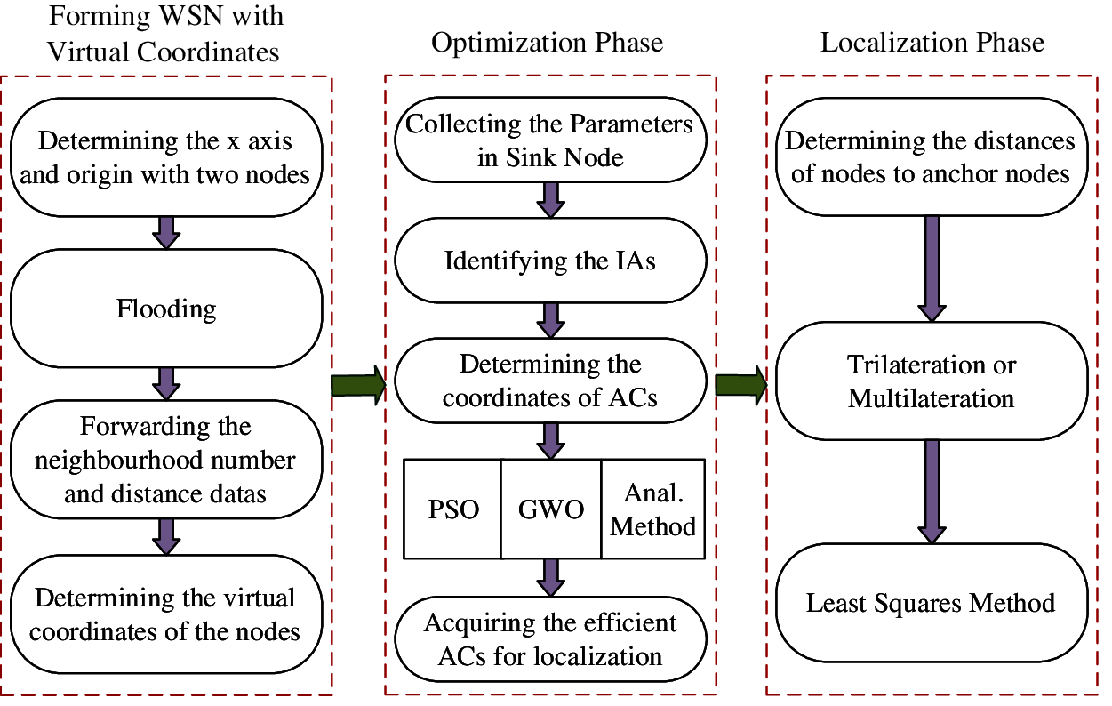
Figure 2: System architecture

4.1 Formation of Virtual Coordinates for Nodes

In this subsection, we show how to build a temporary coordinate system of the wireless network due to the necessity of defining nodes. These nodes have parameter values for determining possible anchor node placement. The modified approach of Capkun et al. [40] is utilized to solve this problem. A randomly chosen node (i) in WSN becomes the origin (0,0) of the temporary coordinate system. If a node (i) in WSN can communicate directly with another node j, i is identified as a one-hop neighbor of j. The following process is executed for every node in WSN:

•   Nodes detect their one-hop neighbors (Ni),

•   They measure the distances to mentioned one-hop neighbors (Di),

•   They measure their battery level (Ei) and speed (Mi),

•   They send Ni, Di, Ei, and Mi to all their one-hop neighbors.

They forward all past neighborhood, distance, and other information in the network to whole forward nodes. So every node in WSN knows its one and two-hop neighbor nodes. They also know the distances between the one-hop and two-hop neighbor nodes. Fig. 3 shows node i and its one-hop neighbors. In this method, two nodes (j,k) are required. Also, i, j, and q must not be in the same line. If we think j node located on the x-axis, k has a positive kx component. So coordinates of those nodes given as follows:

ix=0;iy=0;jx=dij;jy=0; (14)

kx=dikcosγ;ky=diksinγ (15)

So γ , α and β angles are obtained with the following equations:

γ=arccosdik2+dij2−djk22dikdij (16)

α=arccosdil2+dij2−djl22dildik (17)

β=arccosdik2+dil2−dkl22dikdil (18)

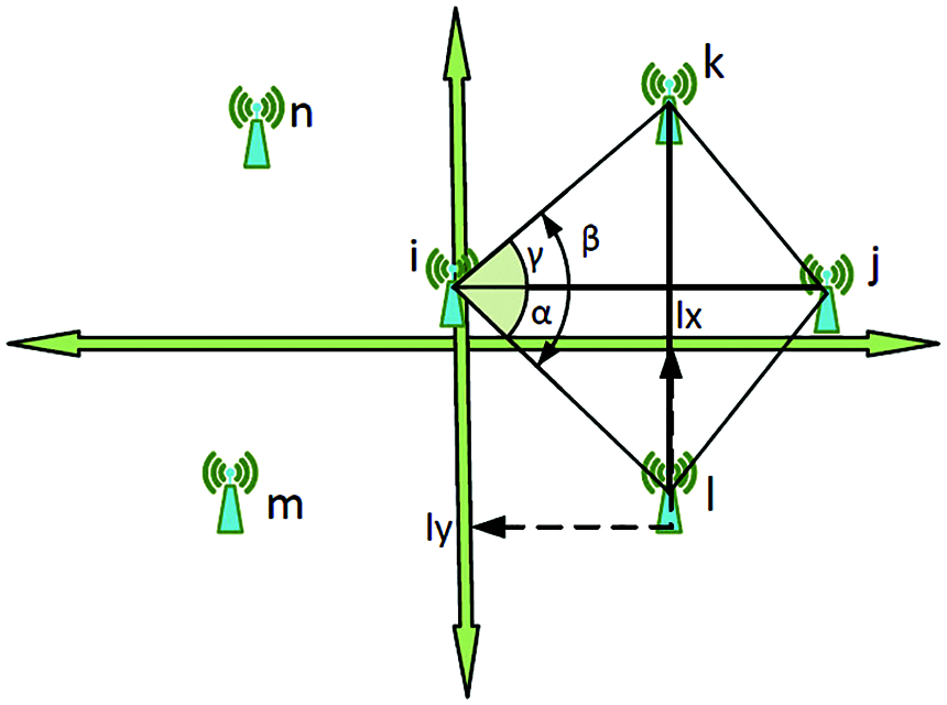
Figure 3: Formation of a one-hop virtual coordinate system

The virtual local coordinate system is built, and all virtual coordinates with other data of those nodes are accumulated in a final sink node thanks to flooding algorithm. After the virtual deployment of nodes with the mentioned method, the system is ready to find optimal anchor placement in WSN.

4.2 Identification of the Anchor Node Candidates

Intersection areas (IA) are the best places for anchor node deployment in WSN. Because it may allow communicating with many unlocalized nodes, namely, anchor nodes in IAs may have a decisive role in many trilateration or multilateration, and they may change of states for more nodes from unlocalized to localized. Sink nodes find the IAs of nodes. It also knows how many nodes intersect for the same IA. It is needed to find the convex closure of nodes. Vertices of the IA are the intersection of two circles. Fig. 4 shows a simple example of the IA between nodes. Those IAs are determined by algorithms like Graham Scan [41].

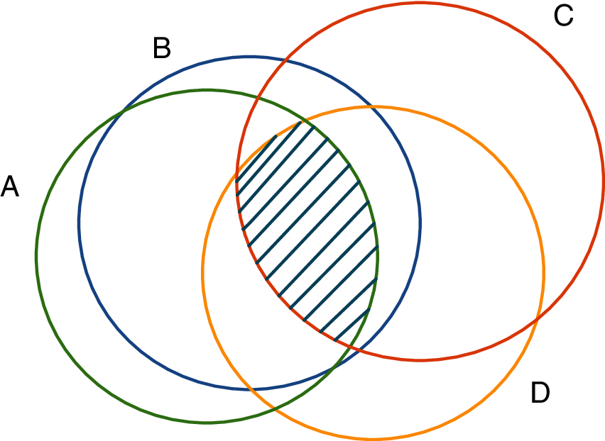
Figure 4: An example of IA for the nodes

There are two situations for the result. Any two nodes in WSN may never intersect or intersect at one point. So, there is no IA for that kind of two nodes. However, the existence of a two-point intersection creates an IA between two circles. Algorithm shows the pseudocode of the IA detection below.

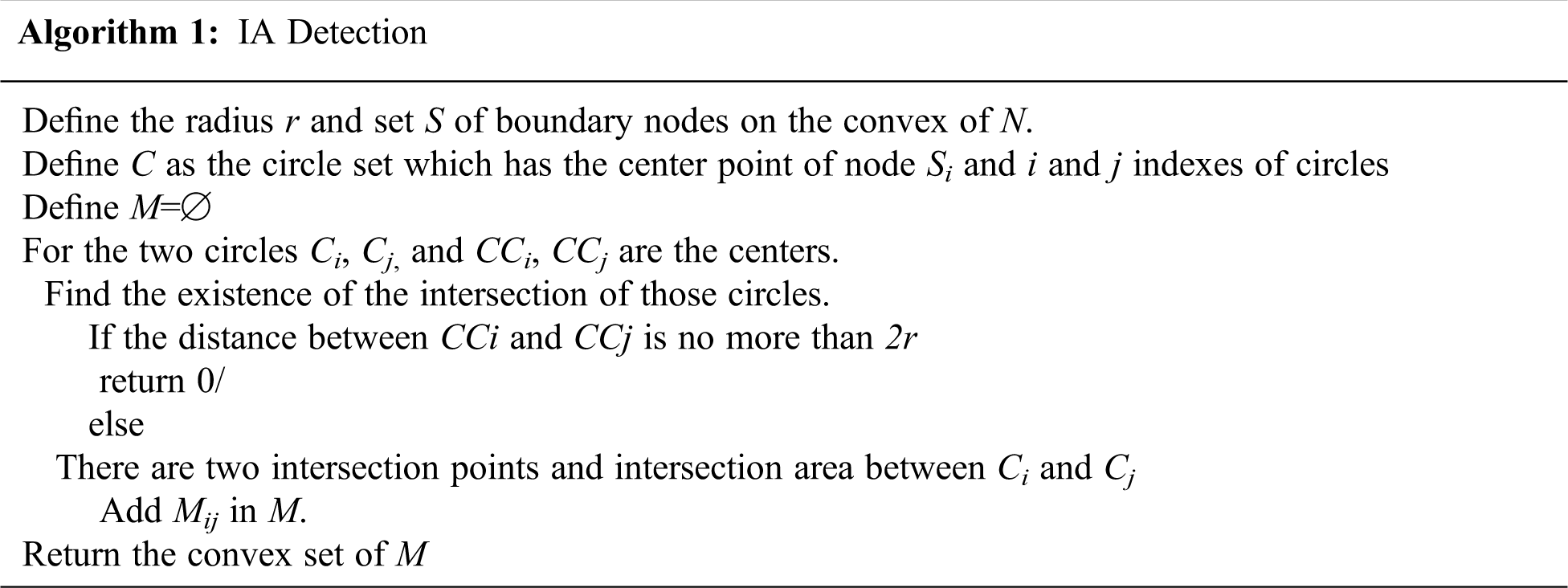
We explain this IA relation between the two nodes in the following equation:

{(xCCi−xCCj)2+(yCCi−yCCj)2<2RIA=1(xCCi−xCCj)2+(yCCi−yCCj)2≥2RIA=0 (19)

In our system model, we defined 3 as a minimum threshold number of nodes for the same IA. For instance, as shown in Fig. 5, if there are IAs between the nodes h and i, h and j and, i and j as pairs, there is an IA of h, i, and j nodes due to 3 paired IA. Also, if there are IAs between the nodes a and b, a and c, a and d, b and c, b and d, and c and d, as pairs, there is an IA of a, b, c and d nodes due to 6 paired IA. Namely, this situation is explained as given below, where t refers to the total node number covers an IA, p is the number of paired or two-noded intersections that include the same IA. If we neglect the negative solution for t :

C(t2)=p (20)

(t−1)t=2p (21)

t2−t−2p=0 (22)

Δ=1−4(−2p) (23)

Δ=1+8p (24)

t=1+1+8p2 (25)

As shown in Fig. 5 α, β, θ, φ, δ, ρ, and γ IAs are in the communication range of 4, 3, 4, 3, 3, 5, and 3 nodes respectively. So the increasing number of connected nodes, which are in the range of IAs, positively affects the extension of iterative localization in WSN. Points in those IAs are candidates to be the places of anchor nodes. We can evaluate those points ( x,y) with two approaches. The first technique is a simple centroid method. The coordinates of those points ( x,y) are obtained as follows:

(x,y)=(x1+x2+x3+…+xnn,y1+y2+y3+…+ynn) (26)

x1 , x2 ….. xn and y1 , y2 ,….., yn are the coordinates of nodes in x and y ordinates, respectively. In addition, the weighted centroid (WC) method is another way to find the mentioned points. The result of the simple centroid is the beginning point of this method. So, ( x,y) is used to determine the weight ( wij) of each node for the weighted centroid method. dij is the measured distance between the node i and the coordinates ( x,y) determined by the simple centroid method. Then, locations of intersection area center points that are found by the simple centroid method. wij can be expressed as:

wij=1dij (27)

Thus, WC algorithm estimates the position of intersection area center points as follows:

Piw(x,y)=∑1n⁡wijPi(x)∑1n⁡wij,∑1n⁡wijPi(y)∑1n⁡wij (28)

n is the total “neighbor node of intersection area center point i . The weight factor is inversely proportional to distance ( dij ). So, the nearest anchor to the initial intersection area center point is found by a simple centroid algorithm in Eq. (26), which will have the most impact in determining the final position of the intersection area center point in Eq. (28). After the determination of intersection area center points in the whole network, GWO and PSO are used to choose the efficient anchor points. While realizing this aim, the fitness function of that optimization method plays a key role. Because fitness of each agent is required, and the best, second, and third wolves or agents are listed in order to those fitness values in the algorithm.

4.3 Generation of Fitness Function for Optimization Methods

The fitness function aims to make more efficient optimization for obtaining more accurate values in localization. For GWO, every wolf in the pack is evaluated based on a fitness function. In this study, the fitness function is established on localization. There are five elements of this fitness function, which can be explained with Fig. 5 initially. All of those parameters are defined by forming a virtual and temporary coordinate system for the whole WSN. Some of them are utilized for the first time in the literature, owing to the absence of determining anchor node positions via metaheuristics methods. The ratio of the average distance of neighbor nodes for the ith AC (dav(i)) to communication range (r) is the first determining value of the function. If it is closer to 1, it contributes to provide an efficient trilateration or multilateration for localization. Energy is another factor in the optimization process. V is the initial voltage level of the battery, Vavi is the average consumed voltage level for the neighbor nodes of the ACi. Less usage of a node is one of the reasons for the long lifetime of a node and also a network. Mobility or speed of neighbor nodes is another variable of the fitness function. Naturally, the speed increase of neighbor nodes may increase the localization error. Thus, if the difference between the maximum speed of a node and the average speed of neighbors for an AC ( Mavi ) gets bigger, fitness function, and the consequent determination of anchor nodes are affected positively. The number of neighbor nodes for ACi is Degi, and its percentage to the whole number in wireless networks is symbolized by Degall that is a sign of to achieve that process generate a useful fitness function for a more efficient iterative localization with selected anchor candidates. As mentioned above, there are two new parameters for the fitness function. Those values are formed to provide more efficient localization. One of those is the number of trilateration which includes the ACi as an anchor. The ratio of that number to all trilateration numbers in networks indicates the effectiveness of the mentioned ACi. After determining the ACs that are in IAs of the nodes via the method in abovementioned pseudocode in and Eq. (19), the sink node saves the lists of the ACs in the communication ranges of nodes. This kind of list can be formed for the WSN in Fig. 5. like the following. a={α}, b={α}, c={α}, d={α,β}, e={β}, f={β,θ}, g={θ}, h={θ,φ}, i={θ,φ}, j={δ,φ}, k ={δ,ρ}, l={δ, ρ, γ}, m={ρ}, n ={ρ}, o={ρ,γ}and p={γ} are the nodes and ACs are in the communication range of them. According to this list, only one node can be localized in the first iteration of the method because it is connected to δ, ρ, and γ as ACs. So there is only one trilateration can be made during the first iteration. The ratio of trilaterations realized by the ACi ( Trii ) to all trilaterations in WSN ( Tri(all) ) is another indicator for the suitability of WSN to localization.

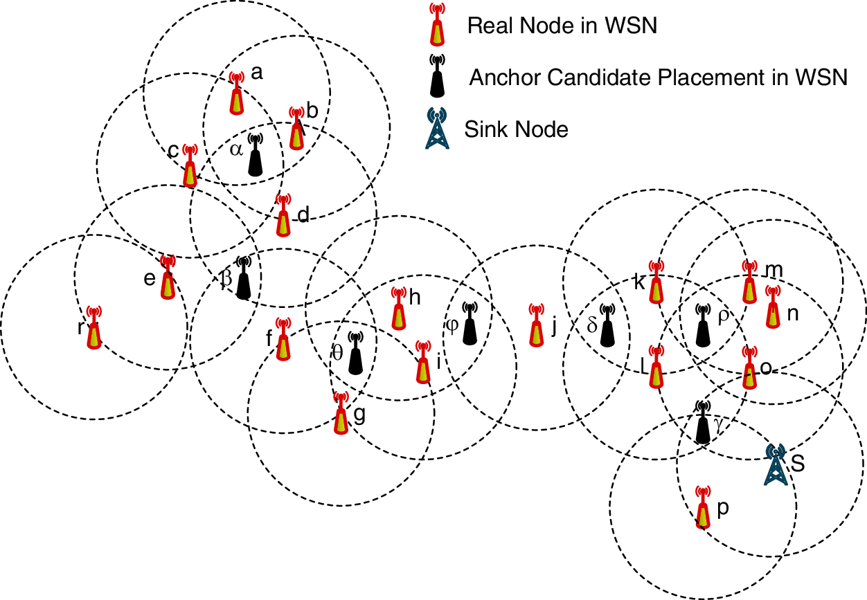
Figure 5: An example of WSN with nodes and anchor candidates. r is the origin, and S is the sink node

As a result of laterations several nodes may be localized. Finally the number of localized number of nodes via the trilaterations made by ACi ( NNodeTrii ), and it’s the rate to the whole node number in a network is an excellent factor to determine how useful iterative localization. It is needed to derive more parameters from obtaining better iterative localization. α1 , α2 , α3 , α4 , and α5 are the numbers in a range of [0,1]. We explain the fitness function in the following equation:

F(x)=α1r−davir+α2V−VaviV+α3Mmax−MaviMmax+α4TriiTri(all)+α5NNodeTriiNNodeAll (29)

After the determination of ACs via mentioned optimization methods, iterative localization is the final step for completing the process for the whole wireless sensor network.

4.4 Localization

RSSI is used as a distance metric for range-based protocols. It is a measured value of received signal power by receiver. Also, it is measured as an integer and can be converted to power unit as dBm. In general, this particular value is obtained by the physical layer of the WSN as in ZigBee nodes. This distance information is used to determine node positions. Examples are locating wireless devices in WLAN and providing location information. This technique can be implemented with a little hardware in a wireless communication system. Simply a receiver gets the power of received signal and it uses these data as the RSSI output for location estimation. RSSI value can be calculated via the following equation:

RSSI=A−10nlog(d) (30)

A indicates the signal strength of transmitter node. In our experiments this value is used as 5 dB. As it is mentioned before n is the path loss of the ambient. d is the measured distance between the transmitter and receiver which is calculated as follows:

d=10(A−RSSI)/10n (31)

RSSI and distance typically have a non-linear inverse relationship such that the RSSI value decreases as the distance is increased. In our study, the least-squares method is performed for the localization process. This kind of mathematical optimization technique has an unknown or target node to locate and n anchor nodes that have coordinates (X1,Y1)……(Xn,Yn). First of all, the distances between the unknown node and anchor nodes are called di . Then a circle is created for each anchor node as a center and has a radius as di . Those circles are intersected in one point that has the coordinates of the unknown node. In this method, at least three anchor nodes are needed. (X1,Y1),(X2,Y2),(X3,Y3)….(Xn,Yn) are the coordinates of the anchor nodes that have distances to the unknown node are d1 , d2,d3……dn. Those distances are explained in the following equations:

{(X−X1)2+(Y−Y1)2=d12(X−X2)2+(Y−Y2)2=d22⋮(X−Xn)2+(Y−Yn)2=dn2 (32)

For the conversion of Ax=B into linear equations:

A=[2(X1−Xn)2(Y1−Yn)⋮2(Xn−1−Xn)2(Yn−1−Yn)] (33)

B=[X12−Xn2+Y12−Yn2+dn2−d12⋮Xn−12−Xn2+Yn−12−Yn2+dn2−dn−12] (34)

x^=(ATA)−1ATB (35)

5  Performance Analysis

In this section, we analyze the performance of the proposed method. We first describe a two-dimensional simulated system model. Then we present and compare the performance results. Also, we investigate the results of the algorithms followed by a detailed discussion.

5.1 Simulated System Model

In this section, we evaluate the performance of the proposed methods. First, a two-dimensional simulation environment is formed with a random defined wireless sensor network, and later, simulation results are presented. In order to test the variable states of the large-scale WSN structure, simulations were performed with the various number of nodes and communication ranges of nodes. In each trial, the nodes are randomly positioned on various network topologies. Naturally, the positions and numbers of anchor candidates have been different each time. In each simulation, the three methods mentioned in the study were executed 1000 times with the topologies that have the same parameters and compared with each other. On the other hand, the proposed methods are compared with Bhatti’s work [42] that provides an efficient evaluation in large-scale WSN localization issue. 5 dB as transmitting power of nodes, 2 as path loss exponent are determiner values of the channel which were used in experimental analysis. In fact, this path loss exponent is the value of the free-space propagation model currently used in our work. Each information packet has 512 bits that is used in info communication. Moving speed of the nodes change between 0-15 m/s. Nodes move periodically with the random walk mobility model in accordance with the mentioned speed limits. In fact, this model is suitable for sheep and cattle movements related to herd localization mentioned in section 1. Other parameters are changed according to experiments. As mentioned before, first of all, anchor node candidates are provided from IAs. There are some technical comparisons to choose from among these kinds of anchor deployment methods. The effect of communication range of node has been observed with the aspects of anchor number and localization error. Changing the node number and processing time of the optimization methods are other subjects that are investigated. This experiment was carried out in MATLAB 2020a environment using a server that has Intel Core I7-9750H processor (2.6 GHz) and 16 gigabyte RAM. Fig. 6 shows an example of WSN with initial and final positions of nodes and anchor nodes.

5.2 Results

5.2.1 Effect of Communication Range

In this section, we evaluate the impact of the communication range on RSSI, anchor node number localization accuracy, and the trade-off options on the number of anchor nodes.

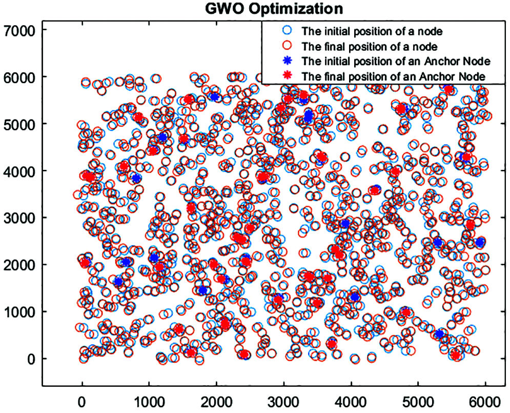
Figure 6: A simulated WSN example with initial and final positions of sensor nodes and anchor nodes are determined by GWO

Fig. 7 shows the received signal strength with respect to the communication distances of the nodes to anchors in our experiments. A consistent decline has been observed for the mean RSSI values via curve fitting method. The distance between anchors and non-localized nodes varies between 0 to 80 m. The RSSI value decreases rapidly from 5 to -15 dB, between 0-10 m communication range. Another decline is also observed between the distances 10-80 m. On the other hand, the rate of the decrease in this region is considerably lower than the first region. The variation of RSS in this second region is about 18-20 dB.

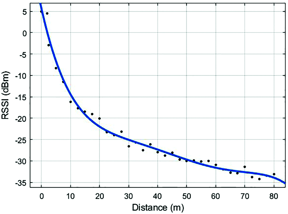
Figure 7: RSSI as a function of the communication distances of the non-localized nodes to anchor nodes

For these experiments which determine anchor node number and other values, four different WSN network structures are considered where 750, 1000, 1250, and 1500 nodes have been placed on a network area of 7500 × 7500 square m Fig. 8 shows the determined anchor node numbers by the PSO, GWO, and Analytical Method versus the communication range of the nodes. While range is increasing, efficient location numbers for anchors rise due to the increment of the IAs. The communication range was changed from 40 to 80 m, with the 5 m steps. In addition, due to the increase in the number of nodes in the WSN from 750 to 1500, the node density and the number of anchor nodes are also increased. This change represents the difference in values between Figs. 8a–8d. As shown in Fig. 8, the PSO method has lower anchor location numbers compared with the other techniques. On the other hand, the GWO method obtained near anchor number values to PSO. Analytical method caused lower performance results.

Figure 8: Minimum anchor numbers for WSNs (a) 7500 m × 7500 m 750 nodes, (b) 1000 nodes, (c) 1250 nodes and (d) 1500 nodes

Furthermore, the difference between the two metaheuristic optimization methods and the analytical method gets bigger with the increment of the communication range of a node. For instance, in the scenario of 750 nodes with a 40-m communication range, anchor numbers are 4.82, 4.82, and 4.88 for PSO, GWO, and analytical method, respectively. However, with an 80-m communication range 41.48, 43.7, and 57.07 values are obtained. In the other three WSNs, those differences between the analytical method and the optimization methods are bigger. For example, the WSN with 1500 nodes that have 40-m communication ranges, 27.71, 28.25, and 34.68 anchors were acquired, while 80-m communication ranges were obtaining 238.1, 249.2 and 331.1 for PSO, GWO and analytical method respectively. Thus, the number of nodes and density of the IAs in a WSN has an essential effect on the performance of the analytical method. Furthermore, it is understood that those parameters have fewer effects on the interoperability of PSO and GWO optimization. Changing the communication ranges of the nodes also affects the localization error. With the pre-selected anchors, localization simulations were executed. As shown in Fig. 9, the differences among the localization results obtained from the four mentioned WSNs are marginal. Furthermore, due to the increment of the node numbers and consequently determined anchor numbers, there is a slow decline observed in localization errors that are shown in Figs. 9a–9d. For instance, those errors change between 8.49-3.66 m, 7.72-2.73 m, 6.72-2.54, and 5.33-2.09 m for WSNs that have 750, 1000, 1250, and 1500 nodes, respectively. It is also observed that GWO anchor deployment-based algorithm has better accuracy, whereas PSO and analytical method algorithms are less accurate for localization. Furthermore, the accuracy of the analytical method is not improved, despite this method has the highest number of anchor nodes. We evaluate the impact of communication range on anchor numbers and localization errors. However, it is not a trivial task to find out which algorithm performs better than the others under different circumstances. To better understand the correlations, we provide multiple charts (See Fig. 10), demonstrating the relationship between localization errors and the number of anchors. In particular, these charts show the trade-off between the density of anchor nodes in a network and localization errors.

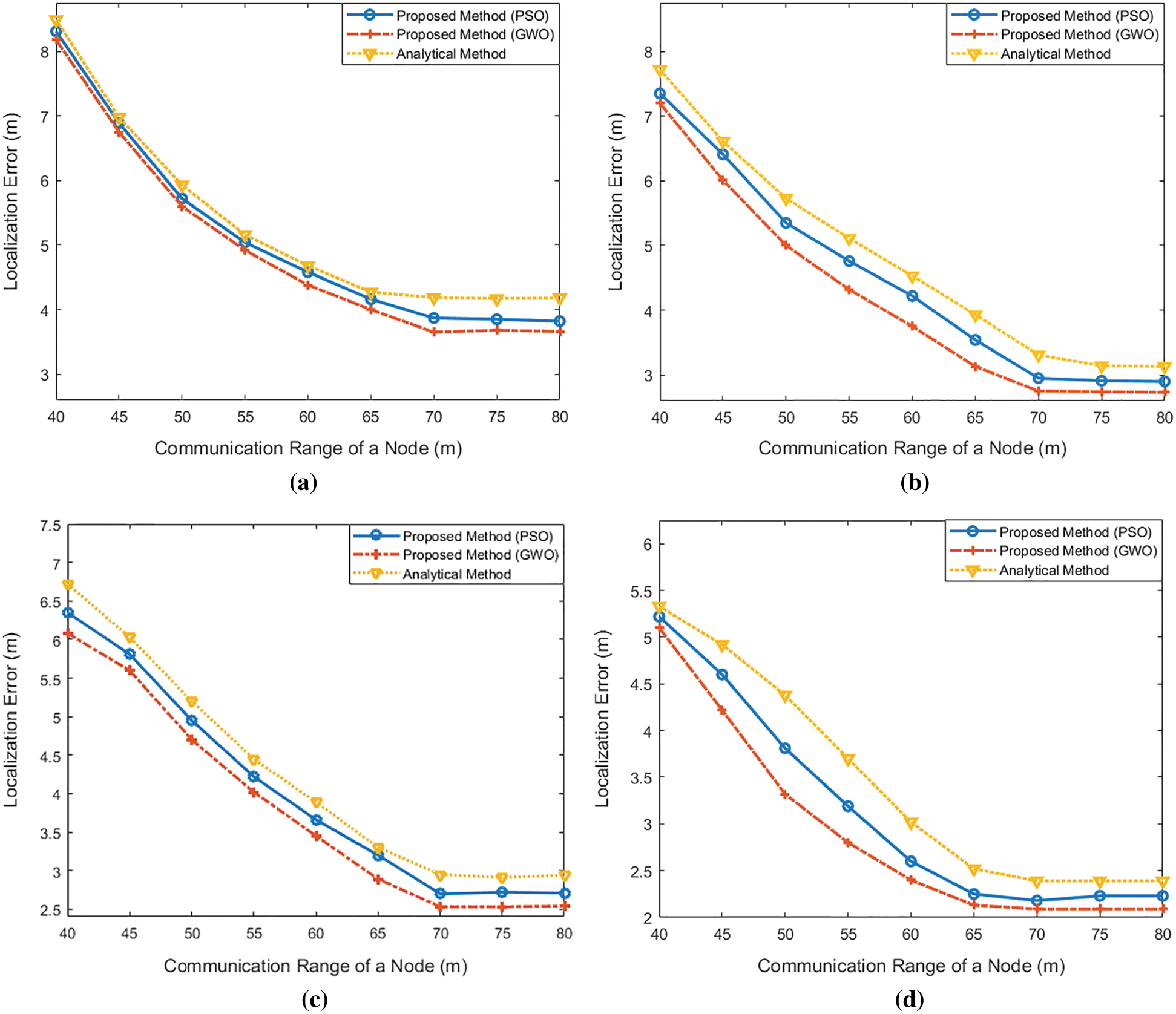
Figure 9: Localization errors with minimum anchor numbers for WSNs (a) 7500 m × 7500 m 750 nodes, (b)1000 nodes, (c) 1250 nodes and (d) 1500 nodes

In these charts, lines that are closer to the origin points represent the algorithms performing better than the others in terms of the aforementioned trade-off. Furthermore, since Fig. 10 reflects the data in Figs. 8 and 9, the changes between Figs. 10a–10d result from these previous graphs. As shown in Fig. 10, the GWO performs better than all other algorithms in terms of localization results. 3.68, 2.75, 2.53, and 2.12 m are the approximate localization error levels that are not affected by the increment of anchor nodes for the GWO method applied to WSNs that have 750,1000,1250 and 1500, respectively. On the other hand, PSO has a relatively steady line and better results compared to the analytical approach, and this makes it a better way to determine the anchors. 3.85, 2.84, 2.7, and 2.24 m are approximate localization error values providing a better trade-off option which are not affected by the increase in the number of anchors.

5.2.2 Effect of Node Number

The number of anchor nodes and localization errors in a WSN depend on the number of sensor nodes if the network size and communication range remains to be unchanged. Fig. 11 shows the relation between the number of nodes in a WSN and localization error. In this simulation, the communication range is 50 m, and the network size is 4000×4000 square meters. The number of sensor nodes vary between 500 and 1000, so the numbers of anchor nodes are determined between 20 and 215, respectively. Localization errors decrease because of the increment of anchor nodes. It is important to note that the marginal inconsistencies in Fig. 11 are emphasized since the RMSE values in the y axis of the chart are displayed in the range of 2.5 and 3.2 despite the fact that these variations have negligible impact on RMSE error results. GWO algorithm obtains slightly better localization results among the three explained methods, and its accuracy changes from 3.01 m to 2.58 m. In addition to this, while running the PSO and analytical method, RMSE errors are decreased from 3.05 meters to 2.63 and 3.14 meters to 2.71, respectively.

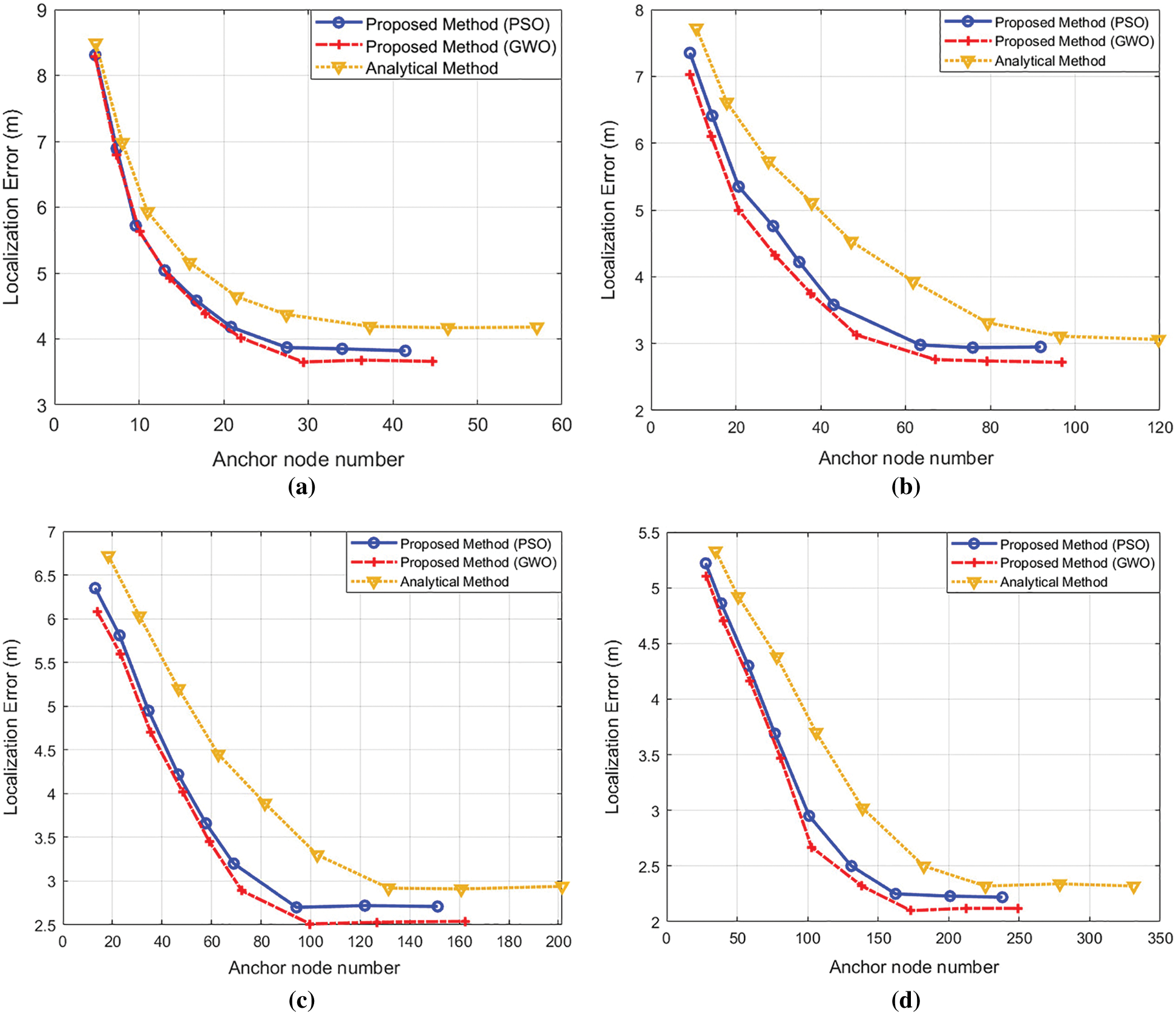
Figure 10: The trade-offs with minimum anchor numbers for WSNs (a) 7500 m × 7500 m 750 nodes, (b) 1000 nodes, (c) 1250 nodes and (d) 1500 nodes

However, still, PSO and GWO are more successful options to determine the anchor nodes in this kind of simulation. For instance, PSO obtains 26.5 as the mean value of anchor nodes in the 500 nodes network. The network under the same conditions provides 26.75 mean value for GWO. Above all, the analytical method leverages 32.78 anchors to provide the abovementioned RMSE results. Similar cases are valid for other simulated networks, and the analytical approach has worse results too. It is evident that the Analytical method is not adequate to be part of an economical option for under those circumstances. GWO and PSO are more useful options to achieve that kind of large-scale WSN localization.

5.2.3 Execution Time of the Algorithms

In a large-scale WSN, optimization methods may take longer time to execute than the deterministic techniques in simulations due to the usage of various parameters for all nodes in the WSN. Thus, the execution times of swarm optimizations have an important role in long and continuous simulations. If it takes too long, it adversely affects the efficiency of the technique. In our experiments, where we measure the elapsed time to run the algorithms the simulation was performed in a 4000 m × 4000 m size network. Also, it has 500 nodes that their communication ranges are 50 meters, like the previous simulation. As shown in Fig. 12, the simulations were performed with 300-1800 seconds time intervals. According to the results, GWO took less time during the simulation.

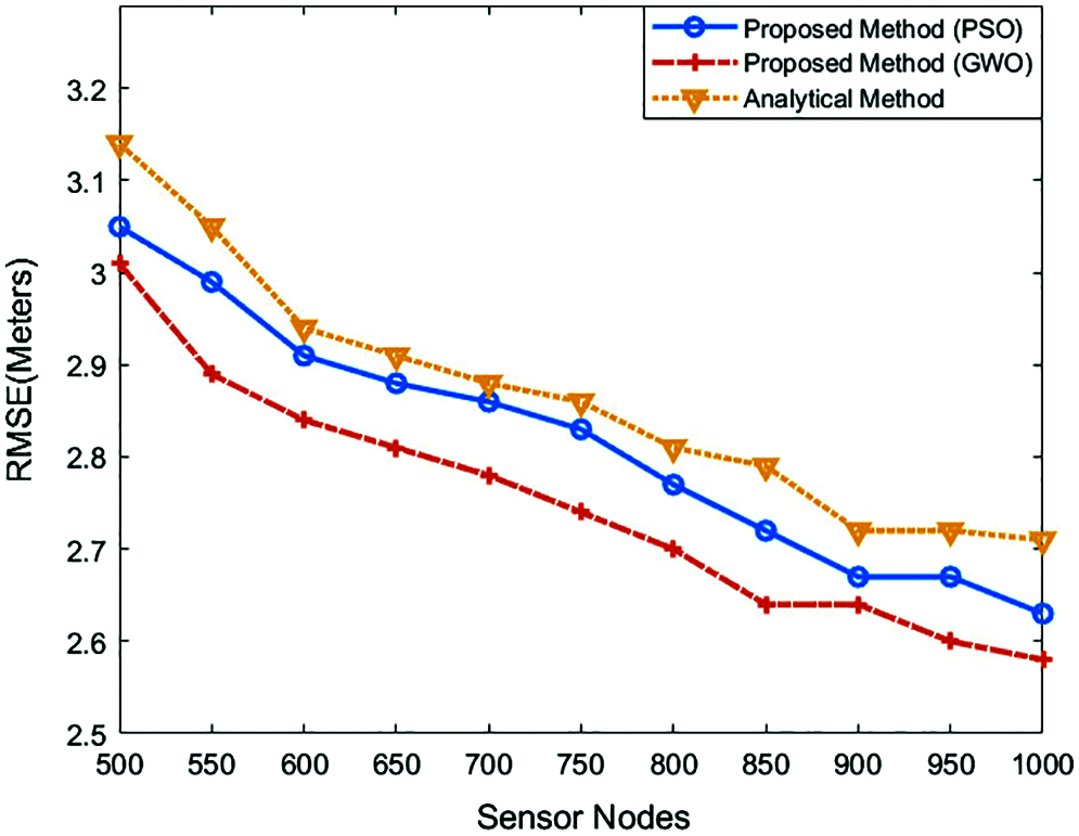
Figure 11: Effect of the changing anchor node numbers to the localization error in a 4000 m × 4000 m WSN

The difference between PSO and GWO is increased as time goes by. The running time of PSO is about 2.55 s during the total simulation time is 1800 s. Hence it may cause a 2.5-second delay in localization for an 1800 second continuous simulation. This value is about 0.98 s for GWO method. We do not compare these algorithms with the analytical method since it is not a continuous process.

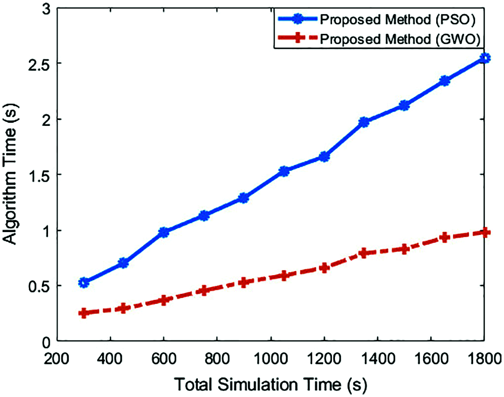
Figure 12: Algorithm execution times of GWO and PSO anchor placement algorithms in a 4000 m × 4000 m WSN for 1800 seconds

5.2.4 Performance Comparison with Machine Learning Methods for Localization

In this subsection, we compare GWO, PSO, and Analytical method with Multiple Regression and Support Vector Machine (SVM) approaches. Also, these machine learning methods are prominent ways to perform the localization process for large-scale WSNs [42]. In that study localization is treated as a regression problem. The impact of varying network parameters, such as anchor population, network size, and localization accuracy of these models are studied in this paper. Also, the effect of anchor distribution types on localization was analyzed. In the first experiment, our goal is to study the localization performance of a WSN in the situation of adding new nodes, whereas the number of anchors is unchanged. Fig. 13a shows this relation. So, the number of nodes is changed between 80-150, in a 100 m × 100 m network area. On the other hand, the number of anchor nodes is 40 for this experiment. GWO, PSO, and analytical method may yield different number of anchor nodes, which could be less than or greater than 40 in some cases. If the number of anchor nodes is more than 40, simulation considers the most efficient 40 anchor nodes and performs localization with those anchor nodes. If the values are less than 40, the simulation gets interrupted, and the results are not taken into consideration. There are two kinds of anchor placement of SVM and Multiple Regression in this experiment. These are random anchor deployment and grid anchor deployment. On the contrary, GWO, PSO, and analytical method can be utilized with random anchor deployment due to the selection of efficient anchor deployment coordinates in a WSN. In this experiment, GWO performs slightly better than PSO, providing 3.4 meters RMSE. Obviously, these two algorithms are more successful than other methods. The localization error of the analytical method rose with the increment of sensor nodes, and it obtains 5.34 meters RMSE. SVM and Multiple Regression have higher localization errors, especially their grid anchor deployment. In grid deployment, RMSEs of those two algorithms increases with the addition of new sensor nodes to. We also analyze the impact of using more anchor nodes while keeping the number of sensor nodes constant. These relations for all mentioned algorithms shown in Fig. 13b. The WSN has 120 sensor nodes in this test. Also, the number of anchor nodes changes between 20-60.

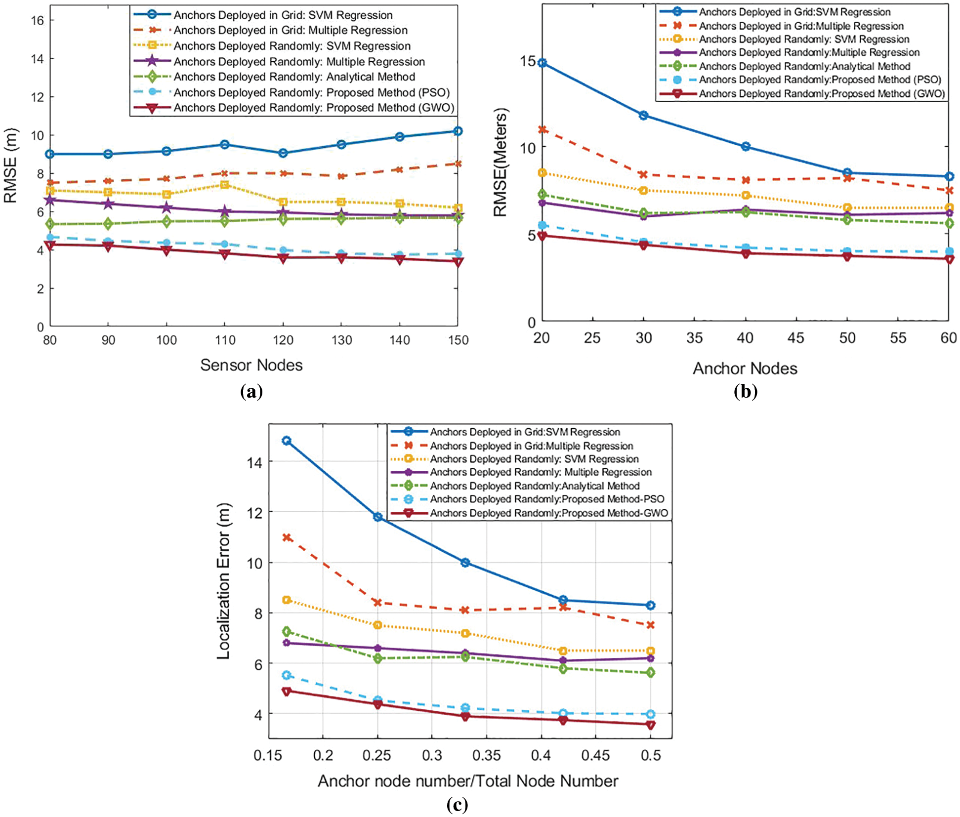
Figure 13: Performance comparison with machine learning methods. (a) Impact of increasing the number of sensor nodes on the localization performances while keeping the number of anchor nodes constant; (b) Impact of increasing the number of anchor nodes on the localization performances while keeping the number of sensor nodes constant; (c) The comparison of the trade-offs between the rate of changing anchor node numbers to all nodes and localization error

According to the results of this experiment, GWO has better results than the other methods, and it achieves 3.58 m as RMSE. Also, PSO performs slightly worse than the GWO based on these results. On the other hand, the analytical method and Machine Learning methods yield the results of 5.62-14.8 m for RSME. Especially machine learning methods with a grid anchor deployment technique can be described as a low-efficient way in this test area. In addition to those circumstances, we would like to analyze the efficiency of localization. This can be better understood with the relation of two parameters that are the rate of anchor node number to the number of sensor nodes and natural localization error. This trade-off is demonstrated in Fig. 13c with the experiment results. GWO has lower RMSE localization errors with the same ratios of anchor node numbers to all nodes in the WSN. With this aspect, GWO is considered to be the most efficient algorithm in this test. Although the performance of PSO is slightly lower than GWO, it has a similar trend in the chart. Also, this kind of anchor deployment method takes advantage of localization when we compare it with the machine learning methods and analytical method. Similar to the previous experiments, grid anchor deployments in SVM and Multiple Regression show the lower performance in this trade-off graph.

5.2.5 Discussion

The proposed GWO and PSO algorithms for the anchor placement problem about localization are successfully compared. The results of experiments show that PSO provides the minimum and the efficient number of anchor node locations for deployment compared to the GWO and analytical method. PSO algorithm is better due to its dynamic optimization. This solution improves the performance of the localization error. On the other hand, GWO has performed minimum localization errors with slightly more anchor nodes than PSO. Both algorithms outperform the localization methods for large-scale WSN environment. When a trade-off chart is formed for both aspects, one can observe that GWO is slightly more efficient than the PSO approach. Finally, our results prove that the GWO method performs better to achieve the minimum localization error with a fair amount of anchor nodes. In contrast, the PSO algorithm revealed fewer anchor nodes for localization. Stability during the change of sensor node number in WSN and less computation time for acquiring the anchor nodes can be considered as additional advantages of the GWO algorithm.

6  Conclusion and Future Work

WSN is a structure that could gather data from various points and use that to activate the environment. Collecting the location information of nodes in WSN is useful that may be utilized in many areas. Thus, the localization process is an essential subject that has two leading roles for nodes in WSN initially. Those roles are non-localized nodes and anchor nodes. Anchor nodes are elements of WSN which have its own location information and may help to localize the non-localized nodes in the network. In the localization process, the existence and efficiency of anchor nodes have an essential role in obtaining accurate location information of nodes. In the first stage, a virtual coordinate system is produced, and nodes are located with the virtual coordinates. During this process, every node in WSN got various information from its neighbors like the distances to one-hop neighbors. Thus every node knows its two-hop neighbors and distances to them. After the formation of the virtual coordinate system, IAs and the coordinates of intersection area center points of the sensor nodes are identified. After that, PSO and GWO optimization algorithms and analytical methods are implemented to choose the minimum and more efficient intersection area center points to put the possible anchor nodes. While determining the locations of anchor nodes, the parameters related to localization formed a fitness function that helps a better optimization. Thus, the iterative localization process is performed with these anchor nodes. GWO and PSO algorithms have never used before for choosing efficient locations to put the anchor nodes. This study utilized GWO and PSO algorithms for determining the most suitable sites to deploy the anchor nodes. The numerical results such as anchor number and running time of algorithm of the proposed GWO method are noted, and it is compared with other techniques such as PSO and Analytical method in anchor deployment stage. In the localization stage, the aforementioned methods are compared with machine learning methods (multiple regression and SVM). Localization error and the trade-off between localization error and anchor numbers were analyzed and compared in this stage as well. In our experiments, many parameters, such as the communication range of a node, size of WSN, and the number of sensor nodes have been changed to obtain the simulation results. According to those results, PSO algorithms have acquired minimum anchor node numbers for localization that is slightly lower than GWO. On the other hand, the GWO technique has provided the most accurate localization among those methods. Also, it has an advantage of simulating in a shorter time when we compare it with the PSO. Some advantages of the study can be listed as follows. Less localization errors were obtained with the applied GWO and PSO optimizations. In addition, both GWO and PSO are suitable methods in terms of multi-criteria decision-making mechanism, as in our study. This method can be performed with newly designed metaheuristic algorithms in the future. Also, GWO can be integrated with other practical metaheuristic algorithms to make a hybrid algorithm with the aim of more efficient anchor node deployment in localization. The theory of the aforementioned study has been successfully applied in large-scale WSNs. On the other hand, optimal anchor placement for 3D WSNs with different parameters is an interesting research question. Furthermore, deploying WSNs in practice to determine the optimal anchor nodes is another worth investigating subject.

Funding Statement: The authors received no specific funding for this study.

Conflicts of Interest: The authors declare that they have no conflicts of interest to report regarding the present study.

This work is licensed under a Creative Commons Attribution 4.0 International License, which permits unrestricted use, distribution, and reproduction in any medium, provided the original work is properly cited.