DOI:10.32604/iasc.2022.020304
| Intelligent Automation & Soft Computing DOI:10.32604/iasc.2022.020304 | |
| Article |
PCN2: Parallel CNN to Diagnose COVID-19 from Radiographs and Metadata
1Department of Computer Engineering, College of Computer and Information Systems, Umm Al-Qura University, Makkah, 21955, Saudi Arabia
2Department of Computer Engineering, College of Computers and Information Technology, Taif University, Taif, 21944, Saudi Arabia
*Corresponding Author: Mohammed Baz. Email: mo.baz@tu.edu.sa
Received: 19 May 2021; Accepted: 01 July 2021
Abstract: COVID-19 constitutes one of the devastating pandemics plaguing humanity throughout the centuries; within about 18 months since its appearing, the cumulative confirmed cases hit 173 million, whereas the death toll approaches 3.72 million. Although several vaccines became available for the public worldwide, the speed with which COVID-19 is spread, and its different mutant strains hinder stopping its outbreak. This, in turn, prompting the desperate need for devising fast, cheap and accurate tools via which the disease can be diagnosed in its early stage. Reverse Transcription Polymerase Chain Reaction (RTPCR) test is the mainstay tool used to detect the COVID-19 symptoms. However, due to the high false-negative rate of this test, physicians usually use chest radiographs as an adjunct or alternative tool. Although radiographs screening is wide-available, low-cost, and its results are timely, relying on radiologists to interpret them manually stands against using radiographs as a diagnostic tool. Motivated by the need to speed up the radiographic diagnosis of COVID-19 and to improve its reliability, this paper proposes a novel deep-learning framework dubbed Parallel Deep Neural Networks for COVID-19 Diagnosis (PCN2). PCN2 treats the radiographs and their metadata simultaneously by running two CNNs in parallel. Firstly: a 2-dimensional CNN (2DCNN) to capture the spatial information from the radiographs due to its super competency in this domain. Secondly, a 1-dimensional CNN (1DCNN) to extract the medical knowledge presented in the metadata. By this integration, PCN2 can make perfect classifications even for those cases in which the infection signs in radiographs are unclear due to being the disease in early-stage, confounded by other markers or overlapped by other diseases. Extensive assessments of PCN2 carried out using several datasets demonstrate average diagnostic accuracy of 99.9 and 0.99 F1-score.
Keywords: CNN; COVID-19 pandemic; radiographs
At the end of 2019, a new generation of Coronavirus named COVID-19 caused by the severe acute respiratory syndrome coronavirus 2 (SARS-CoV-2) surprised the world with its rapid spread and catastrophic impact. The severity of the disease and its serious outbreak steered the World Health Organization (WHO) to declare it as a pandemic. The number of confirmed cases is currently closed to 173 million while the death toll approaches 3.72 million [1]. Recently, several pharmaceutical corporations and research institutions have developed vaccines, and many countries commence vaccination; however, the hope that this pandemic could be finally defeated has been jeopardised by the appearance of several mutants of higher transmissible. This backs the pandemic’s fighting to square one; indeed, some nations face the second or third waves of COVID-19 while others reinforced curfew and lockdown.
The absence of a holistic treatment promotes the desperate needs for fast, cheap, and accurate tools to diagnose the disease in its early stage. However, the key challenge facing rapid diagnoses of COVID-19 is the vast and diverse symptoms presented on patients [2]; while the majority of patients suffer from minor symptoms (e.g., fever, cough, or tiredness), others might have more severe signs (e.g., loss of movement or shortness of breath) or even no symptoms at all. Consequently, diagnosis of COVID19 is typically carried out using Reverse Transcriptase Polymerase Chain Reaction (RT-PCR) that can confide or dispel presence of the antigens of this virus in the respiratory of the suspected cases [3]. RT-PCR requires collecting samples from the nose or throat and then treats them chemically to isolate and identify all known viral genetic variations of the disease. Besides the long-time required by the RT-PCR test to produce the results and the limited availability of its kits in some states, it also suffers from a high false-negative ratio (i.e., the situations in which the tests show that the suspected cases are healthy whereas they are infected). Specifically, several research groups estimate this rate as high as 61% [4–6]; other references show that the maximum accuracy of RT-PCR does not exceed 0.8 and can only be obtained on or after the 8th day of symptom onset [4–6].
With the aim to overcome the critical limitations found in the RT-PCP test, chest radiographs are used as an adjunct or alternative diagnostic tool [7]. The invaluable information encoded in these images allows the physicians to monitor disease progression rather than just determine the infectious status at a single time point, as in RT-PCR. This makes them suitable to diagnose disease and assess its severity [7]. Some medical studies show that chest images of COVID-19 patients share some common signs, such as lesions with ground-glass opacities (GGO), lung consolidation, bilateral patchy shadowing, pulmonary fibrosis, multiple lesions and crazy-paving pattern. Interestingly, other works were able to infer the severity-degree of the disease from the medical images. For instance, Cozzi et al. [8] shows that during the early stage, the peripheral zone of lungs has multiple small patchy shadows and interstitial changes; while during the progression of diseases, multiple Ground-Glass Opacities (GGO) and infiltration start to appear in both lungs and pulmonary consolidation is considered as a sign for a severe case. Nevertheless, one of the key obstructions that stands against adopting radiographs as a diagnostic test is the need to examine each image by a radiologist to decide whether the case is infected or not. Estimations for the time and accuracy of the manual examination show that a cardiothoracic fellowship-trained radiologist takes around a minute on average to examine an X-ray image and that the average diagnostic accuracy is about 78% [9]. This is not negligible time, especially when considering that about 35000 confirmed cases on average are reported daily worldwide.
Inspired by the ability of deep learning to automate the diagnosis of several diseases from their medical images, e.g., arrhythmia, pneumonia, and fundus image segmentation [10–12]. Numerous models were developed to detect COVID-19 cases, e.g., [13–21]. Most of these models employ the Convolution Neuron Networks (CNN) architecture [22] to extract the common visual hallmarks appearing on the radiograph of patients during the training phase; thereafter, the model utilises its gained knowledge to judge new unseen cases. Although these models exhibit high diagnostic reliability, one of the common sources of their performance leakage is inattention of the radiographs’ metadata resources. Annotation, epidemiological history, ages, the clinical manifestation of patients or underlying comorbidities are some attributes that need to be considered when interpreting the radiographs. Several medical studies confirm that the images of patients with different attributes might have different radiographs’ signs; for instance, Chen et al. [23] shows that the image of pediatric COVID-19s’ patients has lower pulmonary lobes with higher bronchial wall thickening than adult patients. Whereas Luo et al. [24] reported that the image features of COVID-19 could not easily be distinguished in the presence of viral pneumonia, Severe acute respiratory syndrome (SARS) and/or Middle East Respiratory Syndrome (MERS) diseases. Furthermore, other works report that some contextual factors (e.g., acquisition parameters, projection-type or even presence of tubes, catheters [25]) might confound the deep learning algorithms.
This paper aims to fill this gap by introducing a novel deep learning model dubbed Parallel Convolution Neuron Networks (PCN2). The underlying approach of PCN2 is to treat the radiographs and their metadata simultaneously by running two CNNs in parallel. Firstly: a 2-dimensional CNN (2DCNN) to capture the spatial information from the radiographs due to its super competency in this domain. Secondly, a 1-dimensional CNN (1DCNN) to extract the medical knowledge presented in the metadata. The key reason for using the 1DCNN instead of recurrent neural networks [22] is the invariance translation property of the convolution operator that enables 1DCNN to interpret the semantic structure regardless of the level of noise usually permeating metadata. Another compelling reason for adopting 1DCNN is being these networks are not confined to fixed-length inputs or outputs; thus, data of variable length can be treated concurrently. The parallel architecture of PCN2 boosts its learning capacity without overwhelming it with excessive learnable parameters; particularly, the parameters space of PCN2 is about a quarter compared to other model which in turn expedites the learning pace and improves its quality. Another key advantage of the parallel architecture is that it allows each CNN to exploit the findings of the other in a complementarity manner to rectify their learning trajectories. This, in turn, allows PCN2 to achieve outstanding results even if some parts of radiographs or their metadata is missing.
According to the best of our knowledge, this is the first work considering using the radiographs’ contextual resources to improve the detection capabilities of the COVID-19. In particular, the key contributions of this work can be summarised as:
1. Develop a novel class of deep learning architecture in which medical reports in conjunction with spatial information (encoded in radiographs) are processed in parallel to enhance detection capabilities of COVID-19. Besides the advantages of this model in rolling out differential diagnoses of this disease, the proposed model paves the path towards building more sophisticated models that can be evolved over time to accommodate updates, e.g., different mutant strains or new diagnosis findings.
2. Reduce the time and computing resources required to train the deep learning model by incorporating the gradually incremental dropout probabilities mechanism for the CNN networks. Specifically, this mechanism achieves this goal by two means; firstly, expedites approaching the most informative partition of a case that is significant to make a clear diagnosis. Secondly, facilitates treating radiographs at their highest possible resolutions by avoiding the use of an image preprocessing technique; hence fine details can be captured accurately.
3. Present comprehensive assessments of the proposed model from different perspectives using several radiographs’ datasets, the results of this assessment demonstrate the high capabilities of PCN2 in diagnosing COVID-19 from radiographs with 99.9 accuracies, 0.99 F1-score.
The remaining of this paper is organised as follows in Section 2 explores the related works and highlights their key contributions. Section 3 discusses the methodology of this work, including a description for the datasets and an overview of the fundamental concepts of the CNN networks. Section 4 presents the proposed models, PCN2, and Section 5 provides the results and discussion. Finally, Section 6 concludes this work.
Scientists and researchers from all disciplines have unified to curb spreading of COVID19 pandemic in all possible ways since its appearance, Artificial intelligence technologists is not an exception; actually, sheer numbers of deep learning models were developed to diagnose the disease from radiographs. Here we review some of these works with the aim to highlight their main contributions and limitations and to point out the merits of our model.
COVIDX-Net [13] is amongst the earliest models introduced to provide fast diagnoses for COVID19 from X-ray images by combining several pre-trained CNN networks with a binary classifier. COVIDX-Net consists of seven models that are: VGG19, DenseNet201, InceptionV3, ResNetV2, InceptionResNetV2, Xception, and MobileNetV2, each of which is trained and tested individually. Evaluation of the model’s performance was conducted over a small dataset consisting of preprocessed 50 X-Ray cases, half of them suffering from COVID-19 using 80:20 training to the testing ratio. The key findings of this study demonstrate the capability of pre-trained models to extract the discriminative features of COVID-19 even over a smaller dataset. Furthermore, it is also shown that VGG19 and DenseNet201 have the highest accuracy of 90%, whereas the lowest achieved accuracy was 50% due to InceptionV3.
Stimulated by the need to improve the diagnosis accuracy using small radiographic datasets, some models employ transfer learning to exploit the knowledge gained from examining individual cases in building a more sensitive classifier. The work in Abbas et al. [14] proposed a three layers framework dubbed Decompose, Transfer, and Compose (DeTraC). DeTraC employs two common pre-trained CNN models: ImageNet and ResNet, to extract the local features appearing in each image individually thereafter passed them to the decompose layer. The underlying approach of this layer is to amplify the irregularities of class boundaries by initiating a sub-class for each distinguished feature found previously. The transfer layer, with the aid of a sophisticated gradient descent optimisation method devised by the authors, retrains the CNN model using these new sub-classes. Finally, the compose layer is used to assemble subclasses into a single binary class stating whether or not the inspected case is infected with COVID-19. DeTraC is evaluated using several datasets comprising 105 COVID-19, 11 severe acute respiratory syndromes and 80 normal samples using 70:30 training to the testing ratio. This evaluation demonstrates that DeTraC can attend up to 95.12% overall accuracy. COVID-ResNet [15] is another example of models aiming to improve the performance of pre-trained CNN architectures by introducing so-called 3-step fine-tune techniques. The underlying concept of this technique is to resize the input radiographs progressively to different sizes and then adjust the learning parameters accordingly. According to the results reported in the original work, COVID-ResNet can achieve 96.23% overall accuracy by employing ResNet-50 as a base network over an unbalanced dataset consisting of 45 COVID-19, 1203 normal, 931 bacterial pneumonia and 660 viral pneumonia patients’ cases. The work proposed in Latif et al. [16] employs 11 pre-trained CNNs including AlexNet, GoogLeNet, DenseNet, Inception, ResNet, VGG, XceptionNet, and InceptionResNet to extract the key features of the X-Ray images, thereafter passing them to a Support Vector Machine (SVM) model which is used to generate the suitable class. The overall accuracy of 95.33% was achieved over a balanced dataset consists of 127 COVID-19, 127 pneumonia and 127 normal images using 60:20:20 training, validation and testing ratio.
Generative Adversarial Networks (GAN) is a contemporary deep learning approach in which new samples can be generated from the ground truth dataset. A GAN architecture comprises two models: a generator that is trained to generate new samples and discriminator that attempts to classify a sample as either a ground truth or a fake (produced by the generator network). Both models compete in a zero-sum game in which the generator endeavours to delude the discriminator about the originality of the sample. The key benefit of GAN in domain of COVID-19 is to generate new samples from a small dataset; hence, the detectability of the model can be improved. The work presented in Khalifa et al. [17] employs the GAN approach alongside transfer learning and augmentation processes to formulate a three-phase diagnosis architecture. In the first phase, both augmentation and GAN are used to generate new samples that are passed to the second phase in which 4 pre-trained models (i.e., AlexNet, GoogLeNet, Squeeznet, and Resnet18) are used train the model, and finally, the third phase is used to test the model. The dataset used in this work consists of -624 X-ray images of two classes, 10% of them are used for training and testing the model, whereas the remaining 90% are generated from the GAN. This work reports that Resnet19 has the highest accuracy of 99% compared to GoogLeNet, AlexNet, and Squeezed.
Waheed et al. [18] demonstrate GAN’s ability to improve the CNN model’s accuracy by more than 10% when they are integrated together, this work firstly introduces a simple CNN constructed from several convolutional layers based on VGG16 architecture followed by the max-pooling and fully connected layers; the model is trained using a small dataset of 331 COVID-19 and 601 normal cases and achieve 85% accuracy. The authors then incorporate this CNN with GAN architecture and allow it to generate 403 of COVID-19 and 721 normal X-ray images; the assessment shows that 95% accuracy can be achieved due to this integration. Another work presented in Loey et al. [19] employs a GAN with three pre-trained models: Alexnet, GoogLenet, and Restnet18 which are trained using two scenarios of 4 and 3 classes of 307 image, including normal pneumonia bacterial, and pneumonia in additional to COVID-19. The results reported in their works exhibit the outperformance of GoogLenet compared to other architectures under 70:20;10 train:test:validation policy.
Building diagnostic models from scratch is another technique that has been introduced in many works; COVID-Net [20] was amongst the pioneer models that adopt this approach. COVID-Net exploits the Projection-Expansion-Projection-eXtension (PEPX) structure of conventional CNN to stack up a large number of convolution layers that can capture meticulous details perfectly. Another crucial advantage of PEPX is its long-range connectivity, which facilities treating large datasets without needing massive computing resources. According to the results reported in this work, 93.3% accuracy level can be achieved over unbalanced dataset comprises 183 COVID-19 cases out of 13,800 total images. Additionally, these results show that the sensitivity of COVID-Net is higher than VGG-19 and ResNet-50 by 32% and 8%, respectively. COVID-CAPS [21] is another bespoke model that exploits capsule networks’ capability in recognising perturbations in the spatial relationships of images. In COVID-CAPS, each layer comprises several capsules, each of which uses its own neurons to capture the common features that are usually appeared in a specific partition of the image. COVID-CAPS employs so-called protocol routing to determine whether or not the desired object is presented in the image. The results shown in this work demonstrate the ability of COVID-CAPS to achieve an accuracy of 95.7% using a simple model consists of 4 convolutional and 3 capsules layers and without using pre-trained model. Tab. 1 summarises some of the key findings reported by the peer works.

This section is devoted to providing the methodology and materials used in this work in two Subsections: 3.1 introduces the dataset used to evaluate the proposed model and Subsection 3.2 overviews the deep learning approach, Convolution Neuron Network (CNN) that is used to develop our proposal PCN2.
The dataset used in this study are adopted from COVID-19 Image Data Collection [26] which includes 328 chest X-ray images of 205 cases whose age range from 12 to 88 years, out of them 253 images are labelled as COVID-19 positive, 2 as healthy, 12 as COVID-19 with Acute Respiratory Distress Syndrome (ARDS), and 61 images are labelled as patients with other diseases including klebsiella, legionella and SARS. This dataset also provides several fields that characterise the cases themselves including demographical data and the observations reported by physicians during their inspection for the radiographs. Besides the finding field that contains the label of the image, the patient_id field contains the unique identifier for the case of the image, the offset field is the number of days since the onset of the symptoms, and the date field records the date on which the image was acquired. These three fields are used jointly to track the progression of the disease of the same case. The age and survival fields store the age of the case and whether they are still alive or not respectively; these two fields, in addition to view field that describe projection type (different Posteroanterior (PA), Anteroposterior (AP), AP Supine (APS), or Lateral (L)) are used as metadata of the image. Another important source of the metadata is the clinical notes field that contains amongst other description for the symptoms and clinical manifestation of the case (Tab. 2). Another dataset used to test the model is COVID-19 Radiography Database [27], which contains many X-ray images collected from several resources and categorised into three classes: COVID-19 positive, healthy, and viral pneumonia whose number of their entities are 1200, 1341 and 1345, respectively. This dataset does not provide any metadata (Tab. 3).


3.2 Convolution Neuron Network Overview
Convolution Neural Network (CNN) is a type of deep learning architecture that has been widely used in those fields related to computer visions [22]; its success in these fields motivated researchers to apply it to other fields, e.g., time series predictions and natural language processing. This section is devoted to overview the basic concepts of CNN using 2-dimensional images as example.
A CNN consists of a set of artificial neurons that are devised to imitate the Biological neurons found in the mammals’ nervous system [22]. Each artificial neuron comprises an activation function that maps inputs to their corresponding output by adjusting two learnable parameters: weights and bias. Typically, these neurons are arranged in layers that are further cascaded to form a deep network. The CNN architecture presented in this work consists of four types of layers: convolutional, nonlinearity, pooling and fully connected that will be reviewed shortly. During this review, we assume that the CNN network consists of
Recalling that the main contribution of this work is to automate the diagnosing of COVID-19 from radiographs by assigning a class to each case, here
Training CNN is accomplished using the backpropagation algorithm [22] which consists of two phases: forward and backwards. In the forward pass, each neuron initialises its weights and biases randomly, then feeds them along with an instance of the training dataset to the activation function that computes the output. The output of a layer is then passed downstream toward the next layer until the final layer is reached and the class of the input is predicated. Thereafter, the error (ϵ) between the predicted values and their corresponding ground truth, denoted here by

The first building block of a CNN is the convolutional layer whose basic concept is that the adjacent pixels of an image are spatially correlated; hence, applying a smoothing operator over neighbouring pixels, e.g., convolution or correlation facilitates recognising the visual structure of objects within images. The input of this layer is a 2-dimensional matrix representing the numerical values of the image’ pixels whereas the weight is several 2-dimensional matrices, each of which is known as a kernel. Convolution is performed between the input matrix and each kernel by placing the top-leftmost cell of the kernel and image over each other, perform a dot product of the overlapped cells and sums up the results, then sliding the kernel row-by-row till its edge arrives at the edge of the image’s bottom-rightmost edge. To illustrate this operational formally, let us assume that we have the
The aggregated output of this layer, dubbed feature map, can be computed by sum values of
Fig. 1 provides a high-level abstraction of the CNN; it is worth noting that the number of the feature maps resulted from a convolutional layer equals the number of its kernels. Moreover, the dimensions of a feature maps are smaller than the dimensions of the original inputs fed into the layer. This characteristic is a direct consequence of applying valid-padding convolution, i.e., passing images as they are to the convolutional layers without expanding their dimension. One of the well-known flaws of valid-padding convolution is the border effect that obstructs resampling the pixels at the edges of the input by the kernel as many as other pixels. Thus, some information at the edges might be lost or under-represented in the outputs of the convolutional layer. One possible remediation of the broader effect is zero-padding [22] that adds new pixels of zero values around inputs’ borders. Two schemes of zero-padding are usually used: half-padding and full-padding; in the former, the number of pixels added into each side of the input equals half of the dimensions of the applied kernel, whereas, in the latter, the full-dimension is used instead. Interestingly, the spatial footprint of input is maintained in the half-padding while increased in the full-padding scheme. The advantage of this enlargement is that it facilitates constructing deeper CNN networks by preventing the rapid collapsing of feature maps resulting from valid padding. Stimulated by this advantage half-padding schemes is employed in this study.

Figure 1: High-level abstraction of the CNN's layers
The nonlinearity layer is the second important layer that is used to amplify the differences found in the feature maps generated from the convolutional layer by passing them into a non-linear activation function, such as hyperbolic tangent (tanh), rectified linear unit or Sigmoid. Most of the activation functions have comparable characteristics; nevertheless, their key difference lies in their ranges; for instance, the range of tanh is
The third main layer of a CNN is the pooling layer, whose key responsibility is to render the features of a feature map over a smaller dimension; thus, treatment of subsequent layers can be more computationally efficient. The pooling layer divides the original feature map into several smaller grids of size
4 The Proposal Parallel CNN to Diagnose COVID-19 from Radiographs and Metadata
PCN2 comprising two types of CNNs: 2-dimensional CNN (2D-CNN) and 1-dimensional CNN (1D-CNN), where the former is used to deal with images and the latter is used to treat the textual data. The numbers of layers in the 2D-CNN and 1D-CNN are 22 and 23 respectively as shown in Fig. 2 which illustrates the block diagram of PCN2. The dimensions of the output of each layer explaining in terms of Width (W), Depth (D) and the number of Channels (C), are given in Tab. 5.

Figure 2: Block diagram of the proposed model, PCN2
As it can be seen in Fig. 2 that PCN2 consists of a 2DCNN and a 1DCNN that are running in parallel to process images and textual resources simultaneously. The main aim of this is to construe visual signs spotted in radiographs in the context of their medical descriptions reported in the associated metadata. Thus, the model can acquire the latent correlations between visual signs and their metadata, which constitutes the medical knowledge required to conduct the classification. The 2DCNN comprises five tuples of “2Dconvolutional-nonlinearity-Droupout-max pooling”. The convolutional layer of the first tuple (2D convolutional-1) comprises 32 kernels of 3 × 3 with ReLU activation function in nonlinearity layer, dropout and max-pooling with the pooling size of 2. The same configurations are used for the subsequent layers except that the number of the convolutional layer’s kernels are doubled after the tuple and the dropout probability is arranged in ascending orders
Moreover, the half-padding convolution strategy has been adopted in this configuration; this can be seen from Tab. 5 as the width and heights of the input and output of each convolutional layer are equal. The key reason for doubling the number of kernels and using the half-padding is to facilitate building throughout deep networks by compensating for the reduction of feature maps generated by the pooling layers. The dropout layer is used to reduce the generalisation error (overfitting error) of a neural network by training multiple instances of the same network, each of which is formulated by removing some nodes randomly. This layer takes a single argument defining the probability of which each node and its connections might be removed from the networks. At test time, this probability is multiplied by the learnable parameters, both weights and bias. Although in a highly dense network with several millions of parameters, it is customary to use a fixed probability across the network; here, we propose a more robust approach in which the value of dropout probability is arranged in ascending orders. As can be seen from Tab. 5, the value of the dropout probability of the first layer is much lower than its peers of other layers; i.e., the dropout probabilities are increased progressively towards the output layer. This approach is defined to quicken the learning pace at the early stage by allowing all nodes to participate in learning and leaving regularisations for further layers with abundant nodes. The flatten layer is used here to reduce the multiple dimensional vectors resulting from processing the images’ spatial features to a sequence of data that suit the dimensionality requirement of the subsequent layers.
The first layer of the 1DCNN is the input layer that reads the metadata of the radiographs to make it available for the one-hot encoded layers. The dimension of the input layer is set at 4000 based on the maximum numbers of characters that a single clinical note field has. The key responsibility of the one-hot encoding layer is to transform each character provided in the input layer into a binary vector of dummy features; thus, the network can work on it mathematically. The length of this variable is adjusted in such a way that allows representing each character uniquely. It is noteworthy that this network is designed based on the approach presented by Zhang et al. [28] in which the learning activities are undertaken at character level rather than at words or sentence. The key advantage of this approach is that it eliminates the need to conduct complicated preprocessing operations (e.g., converted words to lowercase, stemming the words and text enrichment) that are required by other approaches. This, in turn, reduces the computational complexity and memory footprint of the proposed model. The interleaving for the “convolutional, nonlinearity, drop out, and max-pooling” layers is carried out in a similar order that is used to develop 2D CNN. However, the number of kernels in the 1D Convolutional layers are kept fixed, whereas their sizes are doubled after each convolutional layer. A justification for this can be acquired by considering that the textual data, does not like radiographs, differs substantially amongst rows due to using different writing style; vocabularies, and terminologies by different clinicians. This, in turn, requires varying the length of the kernel to extracting the information at different levels of granularity. The concatenate layer is used to connect the outcomes of the upstreaming layers together so that they can be processed jointly by fully connected layers despite their initial different lengths. The inputs to the concatenate layer are the visual and textual features extracted from the radiographs and their metadata by the 2DCNN and 1DCNN, respectively, whereas the output of the concatenate layer is a single dimension tensor of their features. Finally, the fully connected layer is a simple network in which each neuron is connected to all neurons in the next layer; this topology allows each neuron to consider the information gathered in each neuron of the previous layer, which in turn consolidates the learning required to reach a sound conclusion, i.e., provides the posterior probabilities of being an input image belongs to different classes. Here two fully connected layers are used with the aim to deepen the relationships between the spatial and textual findings showing in the data and their corresponding classes. These layers use SoftMax as activation function due to its ability to map a vector of input into a vector real positive number that are required to represent the posterior probabilities.

In this study, PCN2 is deployed on a single machine whose hardware specifications and software environments are given in Tab. 5. Thereafter the weights and biases of all layers in both 2DCNN and 1DCNN are initialised to random numbers that are distributed according to a normal distribution whose parameters are set in accordance with the number of inputs of each layer as proposed in He et al. [29]. Although the ReLU activation function utilised in nonlinearly layers can ameliorate the vanishing and exploding gradients problems, the advantage of using the aforementioned approach is two folds. Firstly, it expedites the convergence of the model to the optimal or near-optimal values by beaking the weights symmetry that might be caused by using the same probability distribution to initialise all the weights of all layers. Secondly, it facilitates deepen the networks without increase the computational loads demanding by the model since the initial values of a layer’s weights are kept consistent with its fans-in. Besides using a robust weight initialising scheme, PCN2 adopts the mini-batch gradient descent scheme; as shown in Tab. 5, the batch size is set to 32. The mini batch differs from other schemes, e.g., batch or stochastic gradient descent schemes, in that the weights of the model are updated in corresponding to the average of gradients of the outcomes of the loss function computed at a portion of the training dataset. This, in turn, allows PCN2 to enhance its features-extraction ability without overburdening it with gigantic inputs at once, as the case in batch gradient descent and to avoid the noisy fluctuations associated with stochastic gradient descent. Another important aspect that is considered when designing and training the PCN2 is to use a simple yet effective strategy to update the learning rate of the gradient descent. Amongst the wide variety of these strategies, the Adaptive Moment Estimation (Adam) due to its ability to improve the learning capacity over sparse gradients, which is the fundamental characteristics of CNN architectures. The next section assessed the effects of these settings on the performance of PCN2 from different perspectives.
Assessment for the accuracy of the proposed model is carried out here by comparing its outcomes to the ground truth data obtained from the dataset. This assessment uses the following statistical measurements: accuracy, precision, recall and F1-score. The definitions of these metrics are given with the aid of the following terms: True Positive (TP), False Positive (FP), True Negative (TN) and finally False Negative (FN). The TP counts the cases classified by both our proposed model and clinicians as patients and TN are the numbers of cases classified by both the model and clinically as healthy. Conversely, FN (FT) signifies the number of cases that our model classifies as patients (healthy), whereas clinicians diagnosed them as (healthy) infected. Based on the above, the accuracy is defined as the ratio of the cases that both the models’ predictions and clinician’s diagnoses are agreed with respect to the total cases seen by the model, which can be expressed mathematically as:
The accuracy metric quantifies the overall effectiveness of a classified as a function of its ability to make true predictions, whether they are positive or negative cases. In the domain of COVID-19, it is highly desired to assess the ability of the model in identifying positive cases so that patients can be isolated early to limit further spreading. Thus, precision and recall are used; the precision is defined as a ratio of those cases classified by the model as true in agreement with physician diagnoses to the sum of the positive class predicted by the model either in agreement or disagreement with physicians. The recall has the same numerator of precision, whereas its denominator comprises the false-negative instead of false-positive as the precision. Expressions for precision and recall are given in Eqs. (2) and (3):
F1-score is a composed metric that is defined as the harmonic mean of precision and recall, i.e.,
The first assessment for the integrity of the proposed model is carried out by quantifying to what extent the proposed approaches used to develop PCN2 affect its learning performance. Two variant models of PCN2 are constructed for the purpose of this assessment. Firstly, SCN2, in which the proposed parallel architecture comprises the 1D and 2D CNNs, is replaced by a single 2DCNN network; hence the input of SCN2 is restricted to the radiographs input without a contextual data in a similar manner that other models reported in the open literature work. Secondly, PCN2v1, in which our approach to gradually increase the dropout probabilities across the layers, is replaced by the scheme that all probabilities are identical, i.e., substituting all dropout layers with dropout (0.5). Finally, a further assessment scenario for the performance of the PCN2 model is conducted by training the model using both radiographs and their metadata and testing it using the radiographs only, i.e., supplying an empty dataset to the 1DCNN during the test phase; this case is referred to PCN2. Both the accuracy as defined in Eq. (4) and the outputs of the loss function (i.e., cross-entropy) of all the above cases are obtained from the simulation sessions at the end of each epoch during the training and test phases and depicted in Fig. 3.

Figure 3: Normalised loss/accuracy of PCN2 and its variants (a) PCN2, (b) PCN2v1, (c) PCN2v2, (d) SCN2
In general, it can be seen that the loss curves of all models decay as more epochs are elapsed, which demonstrate their capability to acquire more knowledge with time. However, the rates at which these curves are decayed, their fluctuations and stopping points differ substantially amongst them. For example, Fig. 3 shows that the rate with which the PCN2 decays are much higher than other curves, i.e., within about 50 epochs, the loss of the model approaches zero. This characteristic can be attributed to being accompanying the radiographs with their metadata empowers the PCN2 with the ability to recognise the cases from different perspectives without using unnecessary learnable parameters which in turn expedites the learning pace and improves its quality. Specifically, the number of the PCN2’s learnable parameters is in order of tenth part compared other modes, e.g., 138 M parameters in VGG [22], 68.1 M in ResNeXt and 60 M in ZfNet. Another notably characteristic of PCN2 shown in Fig. 3 is the narrow generalisation gap, i.e., tiny differences between the loss and accuracy curvesat the training phase and test phase. An explanation for this characteristic can be acquired by considering that the parallel architecture allows each CNN to exploit the findings of the other in a complementarity manner to rectify their learning trajectories. Hence PCNv2 can quickly suit different dataset without consuming lots of time, even if some parts of these data are missing or underrepresented. This claim can be validated further by comparing the curves of PCN2 and PCN2v2, this comparison shows that although the test dataset of PCN2v2 has no metadata, PCN2v2 can get comparable results to PCN2. i.e., PCN2v2 takes about 1.5 times more than the number of epochs required by PCN2 to reach the same loss level.
The benefits of varying dropout probabilities across the layers of both 1D and 2D CNN networks (as in PCN2) over keeping them constant (as in PCN2v1) can be observed by comparing Figs. 3a with 3b. As it can be seen, the loss curve of 3(b) is much noisy than of 3(a); this behaviour can be interpreted by considering the fact that the design philosophy of a deep CNN network is to increase the number of neurons progressively with the depth of the network. Hence the earlier layers of a CNN can capture the primitive features of the image, whereas the latter layers can recognise more detailed features. Hence dropping the neurons of the earlier layers at the same rate as the letter can limit the ability of the model to start learning, which in turn results in fluctuations between different states.
Assessment for the ability of the PCN2 model to make an accurate prediction under different conditions is conducted here by feeding the PCN2 model with three datasets, each of which has a different number of classes. The first dataset [26] comprises four classes (COVID-19, healthy, ARDS and others), the second data have three classes [27] (COVID-19, healthy and other), detailed description for these datasets is given in Subsection 3.1. Finally, the third database is constructed by merging these two datasets randomly and then divided into two mutually exclusive groups, confirmed and COVID-19 negative. The latter group comprises images of those who do not suffer from COVID-19 even if they have other lung diseases, whereas the former group contains all cases diagnosed as COVID-19 patients. These three datasets are passed to the PCN2 and the confusion matrix, i.e., the matrix that shows that TP, TN, FP and FN are given in Fig. 4.

Figure 4: Confusion Matrix of some scenarios (a) Train phase, (b) Train phase, (c) Train phase, (d) Test phase, (e) Test phase, and (f) Test phase
It is obvious from Fig. 4 the proposed model, PCN2, has a high level of prediction accuracy regardless of the number of classes; it can be seen that the lowest readings that our model can achieve is 0.97, whereas the highest is 1. The explanation for this can be acquired by considering that PCN2 employs the concatenate layer to integrate the knowledge gained from the two CNNs together before passing it to fully connected layers that work on them to produce the suitable class for each input. The integration then consolidation architecture of PCN2 allows it to produce high-level quality outcomes without being restricted to the specific number of classes or structure. Fig. 4 also demonstrates that the performance of the proposed model is not affected negatively by the size of the data provided to it. Comparing the readings of the confusion matrix during the training and testing phases shows some neglectable differences amongst them but without any degradations. This characteristic highlight one of the strongest aspects of the proposed model that is its ability to approach the near-optimal situation without a need for lots of samples to practice its knowledge. Our observations in this assessment is of close matching with the learning curves provided in the previous assessment, which shows a small generalisation gap between the train and test sets.
A further assessment for the behaviour of the proposed model is conducted by measuring its performance under a different number of folds using the metrics defined above. Tab. 6 summarises the results of this assessment; the first column of this table is the number of fold and the remaining columns give the average readings recorded from each fold.
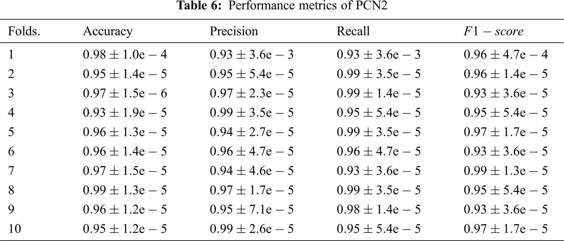
As can be seen from the assessment results that the proposed model, PCN2, exhibits outstanding performance over all cases. This is attributed mainly to the capability of the parallel architecture to exploit the knowledge gained from both radiographs and contextual resources to improve the diagnosis of COVID-19. Another compelling reason for this outperformance is the gradually increasing dropout probabilities across the layer. This approach eliminates a need to employ an image-processing technique which in turn enables PCN2 to extract fine details accurately. Interestingly the outstanding readings of PCN2 demonstrate that it can make accurate classifications even for cases where the infection signs are unclear due to being the disease in early-stage, confounded by other markers or overlapped by other diseases. Hence, 2DCNN can extract the more relevant features to the case, and 1DCNN can find out the pieces of information that are similar to the case under investigation despite the size of the sample fed into the model.
This paper proposed a novel deep learning model dubbed Parallel Deep Neural works for COVID-19 Diagnosis (PCN2) as a tool to aid the diagnosis, prognosis and triage of COVID-19 patients. The underlying approach is to simultaneously treat the images and their metadata by running two CNNs networks of different dimensions in parallel. PCN2 is a flexible architecture in which each CNN network works on a different type of data, but their knowledge is consolidated via the concatenate layer before passing it to fully connected layers that work on them to produce the suitable class. The key advantage of this architecture is that it does not require using a pre-trained model as the case in some related works, e.g., COVIDX-Net or COVIDResNet, which makes its deployment and development incredibly easy. Another main advantage of the PCN2 architecture is that it utilises off-the-shelf frameworks and algorithms; hence its operations do not depend on some bespoke functions that are built especially for it as the case with some pertinent models, e.g., DeTraC or COVID-CAPS. Assessment for the performance of PCN2 from different perspectives demonstrates its ability to find the class of the radiographs with a high level of accuracy and without a need for long training epochs. It is worth noting that this assessment is conducted using a real dataset obtained from medical repositories and not generated using any GAN architecture as the case in some related works, e.g., [15–17]. This is important for combating COVID-19 as it means that PCN2 can be applied directly it can be used directly to triage suspected cases without imposing an overhead. Another important advantage of PCN2 in this regard is that it does not require any preprocessing or postprocessing treatments as the case in some models proposed in the open literature, e.g., [12–13,15] this cannot only leverage the usability of PCN2 but also saves the overhead imposed by these treatments. Besides the above, incorporating the metadata of radiographs in designing PCN2 can pave the path towards building more sophisticated models that can be evolved over time to accommodate updates, e.g., different mutant strains or new diagnosis findings.
Acknowledgement: Taif University Research Supporting Project Number (TURSP-2020/239), Taif University, Taif, Saudi Arabia.
Funding Statement: Funding for this study is received from the Taif University Research Supporting Projects at Taif University, Kingdom of Saudi Arabia under Grant No. TURSP-2020/239.
Conflicts of Interest: The authors declare that they have no conflicts of interest to report regarding the present study.
1. World Health Organization Coronavirus Disease (COVID-19) Dashboard, 09 June 2021. [Online]. Available: https://covid19.who.int/. [Google Scholar]
2. Symptoms of Coronavirus, 09 June 2021. [Online]. Available: https://www.webmd.com/lung/covid-19-symptoms#1. [Google Scholar]
3. D. Axell-House, R. Lavingia, M. Rafferty, E. Amirian and E. Chiao, “The estimation of diagnostic accuracy of tests for COVID-19: A scoping review,” Journal of Infection, vol. 81, no. 5, pp. 681–697, 2020. [Google Scholar]
4. N. Verma, D. Patel and A. Pandya, “Emerging diagnostic tools for detection of COVID-19 and perspective,” Biomedical Microdevices, vol. 22, no. 8, pp. 1–18, 2020. [Google Scholar]
5. F. Bahreini, R. Najafi, R. Amini, S. Khazaei and S. Bashirian, “Reducing false negative PCR test for COVID-19,” International Journal of Maternal and Child Health and AIDS, vol. 9, no. 3, pp. 408–410, 2020. [Google Scholar]
6. S. Mallett, A. Allen, S. Graziadio, S. Taylor, N. Sakai et al., “At what times during infection is SARS-CoV-2 detectable and no longer detectable using RT-PCR-based tests? A systematic review of individual participant data,” BMC Medicine, vol. 18, no. 1, pp. 1–17, 2020. [Google Scholar]
7. R. Yasin and W. Gouda, “Chest X-ray findings monitoring COVID-19 disease course and severity,” Egyptian Journal of Radiology and Nuclear Medicine, vol. 51, no. 1, pp. 1–8, 2020. [Google Scholar]
8. D. Cozzi, M. Albanesi, E. Cavigli, C. Moroni, A. Bindi et al., “Chest X-ray in new coronavirus disease 2019 (COVID-19) infection: Findings and correlation with clinical outcome,” Radiologia Medica, vol. 125, no. 8, pp. 730–737, 2020. [Google Scholar]
9. Northwestern University AI detects COVID-19 on chest X-rays with accuracy and speed: Algorithm outperformed thoracic radiologists in new study, 09 June 2021. [Online]. Available: https://www.sciencedaily.com/releases/2020/11/201124101033.htm. [Google Scholar]
10. L. Sapra, J. K. Sandhu and N. Goyal, “Intelligent method for detection of coronary artery disease with ensemble approach,” in Advances in Communication and Computational Technology. Singapore: Springer, pp. 1033–1042, 2021. [Google Scholar]
11. A. Sharma, K. Guleria and N. Goyal, “Prediction of diabetes disease using machine learning model,” in Int. Conf. on Communication Computing and Electronics Systems, Singapore: Springer, pp. 683–693, 2021. [Google Scholar]
12. F. Pasa, V. Golkov, F. Pfeiffer, D. Cremers and D. Pfeiffer, “Efficient deep network architectures for fast chest X-ray tuberculosis screening and visualisation,” Scientific Reports, vol. 9, no. 1, pp. 1–9, 2019. [Google Scholar]
13. E. Hemdan, M. Shouman and M. E. Karar, “COVIDX-Net: A framework of deep learning classifiers to diagnose COVID-19 in X-ray images,” arXiv: 2003.11055, vol. 1, pp. 1–10, 2020. [Google Scholar]
14. A. Abbas, M. Abdelsamea and M. Gaber, “DeTrac: Transfer learning of class decomposed medical images in convolutional neural networks,” IEEE Access, vol. 8, no. 1, pp. 74901–74913, 2020. [Google Scholar]
15. M. Farooq and A. Hafeez, “COVID-ResNet: A deep learning framework for screening of COVID19 from radiographs,” arXiv: 2003.14395, vol. 1, pp. 1–10, 2020. [Google Scholar]
16. S. Latif, M. Usman, S. Manzoor, W. Iqbal, J. Qadir et al., “Leveraging data science to combat COVID-19: A comprehensive review,” IEEE Transactions on Artificial Intelligence, vol. 1, no. 1, pp. 85–103, 2020. [Google Scholar]
17. N. Khalifa, M. Taha, A. Hassanien and S. Elghamrawy, “Detection of coronavirus (COVID-19) associated pneumonia based on generative adversarial networks and a fine-tuned deep transfer learning model using chest X-ray dataset,” arXiv: 2004.01184, vol. 1, pp. 1–10, 2020. [Google Scholar]
18. A. Waheed, M. Goyal, D. Gupta, A. Khanna, F. Al-Turjman et al., “CovidGAN: Data augmentation using auxiliary classifier GAN for improved Covid-19 detection,” arXiv: 2103.05094, vol. 1, pp. 1–15, 2020. [Google Scholar]
19. M. Loey, F. Smarandache and N. E. Khalifa, “Within the lack of chest COVID-19 X-ray dataset: A novel detection model based on GAN and deep transfer learning,” Symmetry, vol. 12, no. 2, pp. 1–14, 2020. [Google Scholar]
20. L. Wang, Z. Lin and A. Wong, “COVID-Net: A tailored deep convolutional neural network design for detection of COVID-19 cases from chest X-ray images,” Scientific Reports, vol. 10, no. 2, pp. 124–142, 2020. [Google Scholar]
21. P. Afshar, S. Heidarian, F. Naderkhani, A. Oikonomou, K. Plataniotis et al., “Covid-caps: A capsule network-based framework for identification of covid-19 cases from X-ray images,” arXiv: 2004.02696, vol. 1, pp. 1–8, 2020. [Google Scholar]
22. C. Aggarwal, Neural Networks and Deep Learning, 1st ed., NY, USA: Springer, 2018. [Google Scholar]
23. A. Chen, J. Huang, Y. Liao, Z. Liu, D. Chen et al., “Differences in clinical and imaging presentation of pediatric patients with COVID-19 in comparison with adults,” Radiology Cardiothoracic Imaging, vol. 2, no. 2, pp. 1–15, 2020. [Google Scholar]
24. L. Luo, Z. Luo, Y. Jia, C. Zhou, J. He et al., “CT differential diagnosis of COVID-19 and non-COVID-19 in symptomatic suspects: A practical scoring method,” BMC Pulmonary Medicine, vol. 20, no. 1, pp. 1–9, 2020. [Google Scholar]
25. A. Bustos, A. Pertusa, J. Salinas and M. Iglesia-Vayá, “PadChest: A large chest X-ray image dataset with multi-label annotated reports,” Medical Image Analysis, vol. 66, no. 2, pp. 1–12, 2020. [Google Scholar]
26. COVID-19 Image Data Collection, 09 June 2021. [Online]. Available: https://github.com/ieee8023/covid-chestxray-dataset/blob/master/metadata.csv. [Google Scholar]
27. COVID-19 Radiography Database, 09 June 2021. [Online]. Available: https://www.kaggle.com/tawsifurrahman/covid19-radiography-database. [Google Scholar]
28. X. Zhang, J. Zhao and Y. LeCun, “Character-level convolutional networks for text classification,” in Advances in Neural Information Processing Systems. Montréal, Canada, pp. 649–657, 2015. [Google Scholar]
29. K. He, X. Zhang, S. Ren and J. Sun, “Delving deep into rectifiers: Surpassing human-level performance on ImageNet classification,” in IEEE Int. Conf. on Computer Vision, Santiago, Chile, pp. 1026–1034, 2015. [Google Scholar]
 | This work is licensed under a Creative Commons Attribution 4.0 International License, which permits unrestricted use, distribution, and reproduction in any medium, provided the original work is properly cited. |