Intelligent Automation & Soft Computing DOI:10.32604/iasc.2022.020542
Article

Computational Approach via Half-Sweep and Preconditioned AOR for Fractional Diffusion

Andang Sunarto1,*, Praveen Agarwal2,3,4, Jumat Sulaiman5 and Jackel Vui Lung Chew6

1Department Tadris Matematika, IAIN Bengkulu, Bengkulu, 65144, Indonesia
2Harish-Chandra Research Institute (HRI), Prayagraj (Allahbad), 211019, India
3Anand International College of Engineering, Jaipur, 303012, India
4International Center for Basic and Applied Sciences, Jaipur, 302029, India
5Faculty of Science and Natural Resources, Universiti Malaysia Sabah, Kota Kinabalu, 88400, Malaysia
6Faculty of Computing and Informatics, Universiti Malaysia Sabah Labuan International Campus, Labuan F.T., 87000, Malaysia
*Corresponding Author: Andang Sunarto. Email: andang99@gmail.com
Received: 27 May 2021; Accepted: 28 June 2021

Abstract: Solving time-fractional diffusion equation using a numerical method has become a research trend nowadays since analytical approaches are quite limited. There is increasing usage of the finite difference method, but the efficiency of the scheme still needs to be explored. A half-sweep finite difference scheme is well-known as a computational complexity reduction approach. Therefore, the present paper applied an unconditionally stable half-sweep finite difference scheme to solve the time-fractional diffusion equation in a one-dimensional model. Throughout this paper, a Caputo fractional operator is used to substitute the time-fractional derivative term approximately. Then, the stability of the difference scheme combining the half-sweep finite difference for spatial discretization and Caputo time-fractional derivative is analyzed for its compatibility. From the formulated half-sweep Caputo approximation to the time-fractional diffusion equation, a linear system corresponds to the equation contains a large and sparse coefficient matrix that needs to be solved efficiently. We construct a preconditioned matrix based on the first matrix and develop a preconditioned accelerated over relaxation (PAOR) algorithm to achieve a high convergence solution. The convergence of the developed method is analyzed. Finally, some numerical experiments from our research are given to illustrate the efficiency of our computational approach to solve the proposed problems of time-fractional diffusion. The combination of a half-sweep finite difference scheme and PAOR algorithm can be a good alternative computational approach to solve the time-fractional diffusion equation-based mathematical physics model.

Keywords: Time-fractional diffusion; half-sweep; finite difference discretization method; preconditioned accelerated over relaxation algorithm

1  Introduction

The increasing interest in the application of fractional-order partial differential equations (FPDE) to replace the classical integer-order partial differential equations can be seen obviously in recent years. The fractional derivative terms in the FPDE, which have many extraordinary things yet to be discovered, has attracted the attention of worldwide mathematics experts. Dealing with the research in fractional calculus is crucial these days because the research gap is still wide open. Although the standard theory is already presented to give us the correct results, the new FPDE problems keep coming and causing the standard theory to be modified or extended. This work is motivated by the recent active development of an accurate and efficient numerical approach to solve FPDE. Generally speaking, there are three types of FPDE, namely time-fractional, space-fractional, and time-space-fractional differential equations. These FPDEs can be distinguished based on the presence of fractional derivative, which either on time derivative, space derivative or both time and space derivative. In this paper, time-fractional type is the subject of interest and an investigation on developing an efficient computational approach for time-fractional diffusion equation is conducted.

In recent years, the time-fractional diffusion equation (TFDE) has been actively applied in many fields. Li et al. [1] used TFDE to improve signal smoothing performance in signal processing. Then, González-Olvera et al. [2] applied TFDE to obtain a better result in the simulation of shipping water events compared to the classics diffusion equation. Next, Liao et al. [3] developed a TFDE based image denoising model. Furthermore, TFDE exists in many mathematical models such as pattern formation [4], groundwater pollution [5], contaminant transport [6], option pricing and risk calculation [7], and methyl alcohol mass transfer in silica [8]. To better understand and make an accurate interpretation of these TFDE models, the solution of the models must be computed accurately and efficiently using a computational approach. The solution of a TFDE is dependent on the fractional order since the fractional order influences the concentration of the diffusion process. For instance, when the fractional order is ranged within (0,1) , the diffusion is slow, which also known as a sub-diffusion phenomenon. Whereas when the fractional order is (1,2) , the diffusion is fast or known as super-diffusion phenomena. Besides that, several fractional operators have been introduced to facilitate the research on solving the TFDE significantly, referred to in de Oliveira et al. [9]. These fractional derivatives can be categorized into the classics and the moderns. The classics fractional derivatives include Grunwald-Letnikov derivative, Liouville derivative, Caputo derivative, Hadamard derivative, Marchaud derivative, Miller-Ross derivative, Weyl derivative and Erdelyi-Kober derivative. Meanwhile, the modern fractional derivatives are like Coimbra derivative, Hilfer derivative, Davidson derivative, Chen derivative, Atangana-Baleanu, Caputo-Fabrizio, and many more. More details about the classification of fractional operators can be seen in Baleanu et al. [10].

The present paper is devoted to investigating the numerical solution of a TFDE using an innovative finite difference scheme and an efficient computational algorithm. Solving TFDE using a numerical method has become a research trend nowadays since analytical approaches are quite limited. Many numerical methods have been proposed to solve TFDE. However, based on our preliminary study, we found that the usage of a finite difference method to solve TFDE needs to be explored, especially in terms of efficiency to obtain the solution. In the past, [11] used the explicit finite difference method to solve TFDE. Then, Murio [12] used the implicit finite difference method to obtain an unconditionally stable numerical solution to TFDE. Another unconditionally stable numerical method called Crank-Nicolson finite difference method has been applied on TFDE [13]. Recently, an innovative finite difference scheme called the half-sweep finite difference (HSFD) with iterative method emerges as a potential approximation to TFDE [14]. We are interested to apply a HSFD because it is a good computation complexity reduction approach. The advantage of using HSFD over the standard finite difference method to solve several mathematical models can be seen in the literature. It is worth to mention that HSFD has been applied to efficiently solve linear partial differential equation [15,16], nonlinear partial differential equation [17], and fuzzy partial differential equation [18].

This paper extends the work from [14] by achieving a high convergence rate of the solution. A preconditioned technique is proposed and integrated with an accelerated over relaxation (AOR) iterative method introduced by [19]. The contribution of this paper is to present a preconditioned accelerated over relaxation (PAOR) algorithm via an HSFD scheme to solve a one-dimensional TFDE efficiently. Throughout the formulation of an HSFD approximation, a Caputo derivative is applied to approximate the time-fractional term in the equation. This efficient numerical method will increase the literature for the researchers to better understand the time-fractional mathematical model of equilibrium, stability, and time evolution in the long-time limit [20,21]. The details about our numerical method are described in the following sections.

2  Numerical Method

2.1 Half-Sweep Finite Difference with Caputo Derivative

In this section, an HSFD approximation with Caputo derivative is formulated by considering a general form of TFDE as follows:

∂αW∂tα=p∂2W∂x2+q∂W∂x+rW. (1)

Based on Eq. (1), W=W(x,t) is the solution function, and we assume it exists in the domain subjects to the Dirichlet boundary conditions. Then, p,q and r are either known functions or coefficients. The degree of fractional order for Eq. (1) is denoted by α . The present paper investigates one-dimensional TFDE with 0<α<1 , which is a sub-diffusion problem. This range of fractional order is extended from the classic diffusion equation, which has the value of the time fractional order α=1 , by considering all rational numbers between 0 and 1. More details about TFDE, particularly unconventional diffusion theory, can be referred to in Evangelista et al. [22].

Definition 1. Caputo derivative is defined as

∂α∂φαf(φ)=1Γ(m−α)∫0φf(m)(τ)(φ−τ)α−m+1dτ, (2)

where m−1<α≤m, α>0 and φ>0 [23].

Using Def. 1 as shown in Eq. (2), the time-fractional term in Eq. (1) can be approximated by

∂αW∂tα=1Γ(1−α)∫0∞∂W(xi,τ)∂t(tj−τ)−αdτ,0<α<1, (3)

and form a discrete approximation that can be written as

∂αW∂tα≅σα,k∑n=1Nωn(α)(Wi,j−n+1−Ui,j−n), (4)

where

σα,k=1Γ(1−α)(1−α)kα, (5)

and

ωn(α)=n1−α−(n−1)1−α. (6)

Next, for the HSFD discretization on the space derivatives, we consider a partitioning of the solution domain that is uniformly so that the grid framework is fixed everywhere. We denote h=H/M for the space domain [0,H] and M +1 points. For the time step, we denote k=T/J for the time domain [0,T] and J+1 levels. Therefore, the value at each point is denoted by W(x,t)=W(xi,tj)=Wi,j for i=0,1,2,3…,M, and for j=0,1,2,…,J . The application of HSFD on the spatial derivatives of Eq. (1) combining with the Caputo time derivative as in Eq. (4) produces

σα,k∑n=1Nωn(α)(Wi,j−n+1−Wi,j−n)=p8h2(Wi−2,j−2Wi,j+Wi+2,j)+q4h(Wi+2,j−Wi−2,j)+rWi,j, (7)

for i=2,4,6,…,M−2 .

When the Caputo-HSFD approximation as in Eq. (7) is applied at j≥2 , for instance, the equation can be expressed in the form of

σα,k∑n=1Nωn(α)(Wi,j−n+1−Wi,j−n)=p~Wi−2,j+q~Wi,j+r~Wi+2,j, (8)

where p~=p8h2−q4h,q~=r−p8h2,r~=p8h2+q4h.

By letting j=1 in Eq. (7), a linear equation which represents the first level of the solution of TFDE is expressed as

−p~Wi−2,1+q~Wi,1−r~Wi+2,1=Fi,1, (9)

where Fi,1=σα,kWi,1 . With M+2 grid points to be numerically computed, a system of linear equations can be generally formed as

ΩW∼=F∼, (10)

where

Ω=[q~2−r~2−p~4q~4−r~4−p~6q~6−r~6⋱⋱⋱−p~M−4q~M−4−r~M−4−p~M−2q~M−2]((M2)−1)2, (11)

W∼=[W2,1W4,1W6,1⋯WM−4,1WM−2,1]T, (12)

and

F∼=[F2,1+p~2W0,1F4,1F6,1⋯FM−4,1FM−2,1+r~M−2WM−2,1]T. (13)

2.2 Analysis of Half-Sweep Finite Difference Stability

In this section, the stability of Caputo-HSFD approximation as in Eq. (7) is analyzed using both the Von-Neumann method and the Lax equivalence theorem [24,25].

Theorem 1

The Caputo-HSFD approximation to (1) with 0<α<1 on the finite domain 0≤x,t≤1 , with zero boundary condition W(0,t)=W(H,t)=0 for all t≥0, is unconditionally stable.

Proof:

Defining Wi,j=ξjei(ωih) and ω is an element of a real number. Eq. (7) can be derived using ξjei(ωih) into

σα,kξj−1ei(ωih)−σα,k∑n=1Nωn(α)(ξj−n+1ei(ωih)−ξj−nei(ωih))=−p~ξjei(ω(i−2)h)+(σα,k−q~)ξjei(ωih)−r~ξjei(ω(i+2)h), (14)

and can be reordered into a more straightforward discrete equation in the form of

σα,kξj−1−∑n=1Nωn(α)(ξj−n+1ei(ωih)−ξj−nei(ωih))=ξj(((−p~−r~)cos⁡(ωh))+(σα,k−q~)). (15)

Since

ξj=ξj−1+∑n=1Nωn(α)(ξj−n−ξj−n+1)(1+(p~+r~)σα,kcos⁡(ωh)+q~σα,k), (16)

and

(1+(p~+r~)σα,kcos⁡(ωh)+q~σα,k)≥1, (17)

for any values of α,n,ω,h and k , we have an inequality that can be expressed as

ξj≤ξj−1+∑n=1Nωn(α)(ξj−n−ξj−n+1),n≥2. (18)

By letting n=2 as in Eq. (18), we obtain

ξ2≤ξ1+ω2(α)(ξ0−ξ1), (19)

and in general, Eq. (19) becomes

ξj≤ξj−1, j=1,2,…, (20)

or

ξj≤ξj−1≤ξj−2≤…≤ξ1≤ξ0. (21)

Thus, it follows that the solution of TFDE being approximated by using the Caputo-HSFD approximation equation converges to an exact solution as h,k→0.

2.3 Preconditioned Accelerated Over Relaxation Iterative Method

This section discusses the formulation of the PAOR iterative method based on the Caputo-HSFD approximation. Using the linear system as in Eq. (10), a conversion of an original linear system into a preconditioned one can be done as follows:

Ω∗Ψ∼=F∗∼, (22)

with a new coefficient matrix,

Ω∗=PΩPT, (23)

a preconditioned right-hand side vector,

F∗∼=PF∼, (24)

and a new approximation

W∼=PTΨ∼. (25)

Based on this system conversion, a preconditioned matrix P, that we proposed is [26]:

P=I+S, (26)

where

S=[0−s2000000−s4000000−s60000⋱⋱⋱000000−sM−4000000], (27)

and matrix I, is an identity matrix.

Next, we consider the matrix Ω∗ as a summation of three matrices. The three matrices, D , L and V , represent the diagonal, the lower and the upper triangular matrices, respectively. The matrix Ω∗ can be expressed as [27,28]:

Ω∗=D−L−V. (28)

Using Eqs. (22) and (28), the PAOR iterative method based on Caputo-HSFD approximation can be formulated into

Ψ− (K+1)=(D−ωL)−1[ (ρ−ω)D+ρV+(1−ρ)D ]Ψ− (K)+ρ(D−ωL)−1F*-, (29)

where ω and ρ are the parameters for accelerating the convergence rate of the solution. We name Eq. (29) as the HSPAOR method for simplicity. The algorithm for the HSPAOR method is provided as in Algorithm 1.

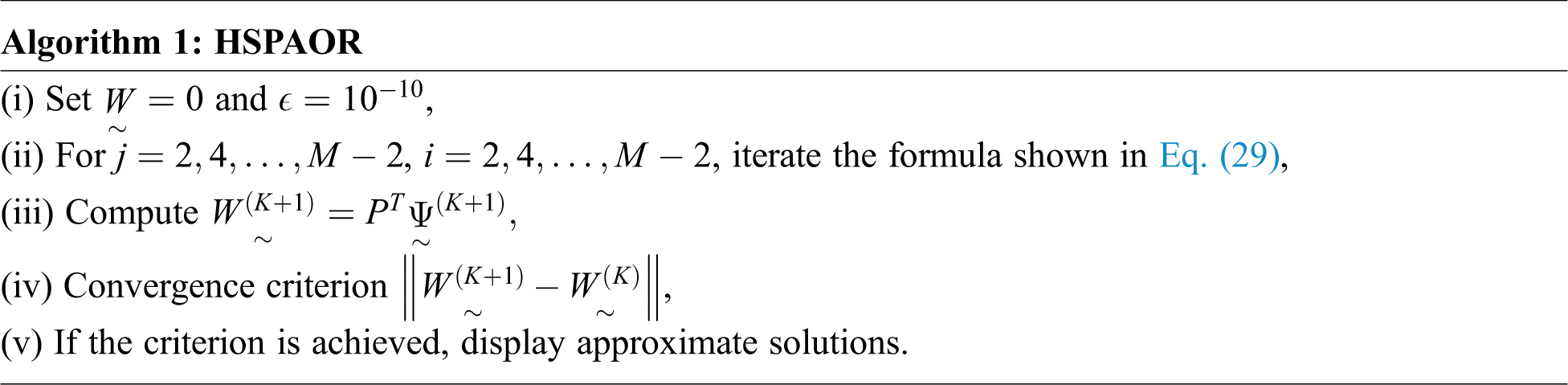
2.4 Convergence Analysis of HSPAOR Method

In this section, the analysis of convergence of the HSPAOR iteration process is presented. The iterative matrix for HSPAOR can be expressed in the form of

Aω,ρ=(D−ωL)−1[(ρ−ω)D+ρV+(1−ρ)D]. (30)

Theorem 2

If the HSPAOR iteration converges or spec(Aω,ρ)<1 for some ρ and ω≠0 , then one of the following statements hold:

(i) ω∈(0,2) and ρ∈(−∞,0)∪(0,+∞),

(ii) ω∈(−∞,0)∪(2,+∞) and ρ∈(2ω(2−ω),0)∪(0,2) .

Proof:

Suppose the eigenvalues λj of Aω,ρ are connected with the eigenvalues ξj of Sω,ω≡Sω . Note that Sω is a SOR iteration matrix by

λj=(1−ρω)+ρωξj, (31)

where j=2(2)J−2. Also, note that

∏j=2,4,..J−2ξj=(1−ω)j. (32)

Using Eqs. (31) and (32), we have

∏j=2,4,..J−2(1−ωρ+ωλjρ)−(1−ω)j. (33)

Since |λj|<1 for j=2(2)J−2 ,

<∏j=2,4,..J−2(|1−ωρ|+|ωρ|)=(|1−ωρ|+|ωρ|)j, (34)

which can be expressed in a simpler way as

|1−ω|<|1−ωρ+|ωρ||. (35)

Eq. (35) is equivalence to

|ρ(1−ω)|<|ρ−ω|+|ω|. (36)

Hence, it can be shown Eq. (36) holds if and only if exactly one of the following statements hold:

(i) ω∈(0,2) andρ∈(−∞,0)∪(0,+∞),

(ii) ω∈(−∞,0)∪(2,+∞)and ρ∈(2ω(2−ω),0)∪(0,2) .

Theorem 3

If the HSPAOR iteration with ω=0 converges or (spec(A0,ρ)<1) , then 0<ρ<2.

Proof:

If ω=0, then

A0,ρ=(1−ρ)D+ρ(L+U). (37)

If μj,j=2(2)J−2 are the eigenvalues of some iteration matrix B , then the eigenvalues λj of A0,ρ is

λj=1−ρ+ρμj, (38)

which implies

μj=1ρ(ρ−1+λj), (39)

where j=2(2)J−2.

By letting B=0 , we get

∑j=2,4,..J−2μj=0=∑j=2,4,..J−21ρ(ρ−1+λj). (40)

From Eq. (40), we have

∑j=2,4,..J−2λj=(J2−1).(1−ρ), (41)

and consequently

|(J2−1)(1−ρ)|=|∑j=2,4,..J−2λj|≤∑j=2,4,..J−2|λj<n,|. (42)

Since |λj|<1, from the hypothesis, therefore,

|(J2−1)(1−ρ)|<n, (43)

and the proof is completed.

3  Results and Discussion

In this section, two TFDE test examples are considered for evaluating the efficiency of the HSPAOR method. The benchmark used is the previously developed method of PAOR from [29]. The three criteria, namely the number of iterations, computation time in simulation program (measured in seconds or sec.) and maximum absolute error, are compared to each other at three different orders of α values, i.e., α=0.25,α=0.50 and α=0.75 . The cycle of iteration process in Algorithm 1 stops at ε=10−10 . Below are the following two TFDE examples:

Example 1: We consider a TFDE in the form of [30]:

∂αW∂tα=∂2W∂x2. (44)

To initiate the simulation, we set the initial condition

W(x,0)=x2, (45)

and the Dirichlet boundary condition is stated as follows

W(0,t)=2ktαΓ(α+1),W(H,t)=H2+2ktαΓ(α+1). (46)

Example 2: We attempt to solve the following TFDE [31]:

∂W∂t=Γ(1.2)xβ∂βW∂xβ+3x2(2x−1)e−t. (47)

We initiate the approximate solution's computation using the initial condition

W(x,0)=x2−x3, (48)

and used zero Dirichlet condition. The exact solution is given by

W(x,t)=x2(1−x)e−t. (49)

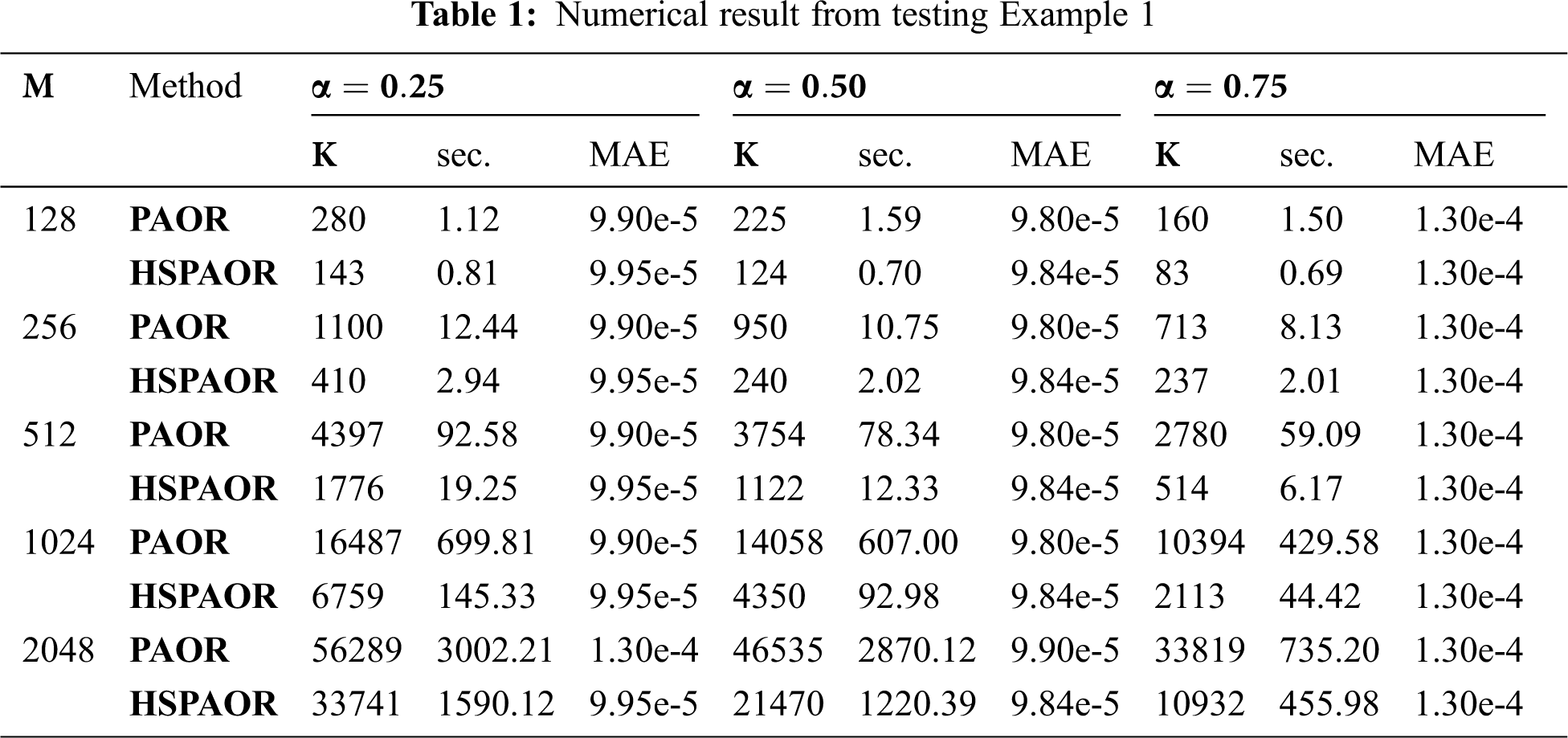
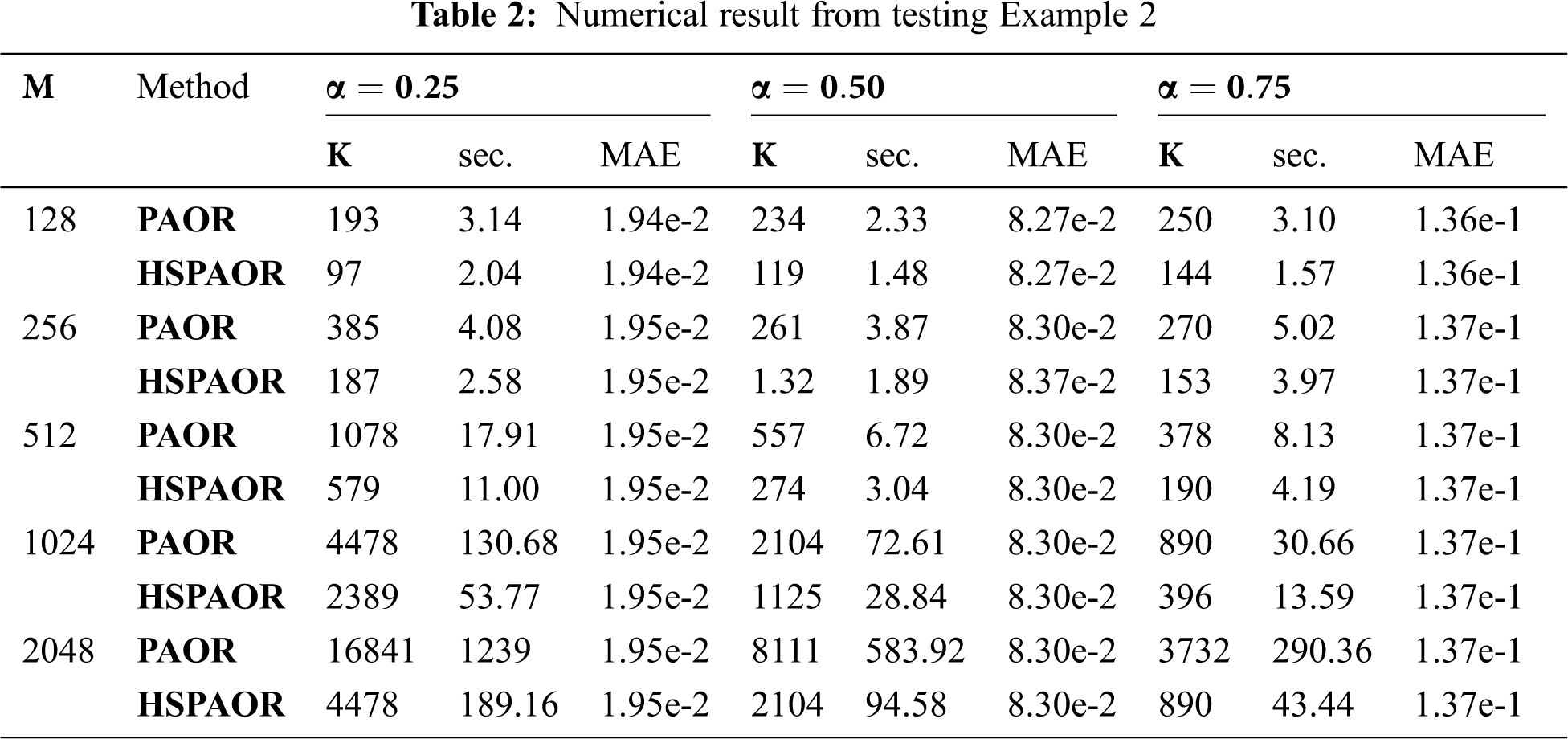
The numerical results from both HSPAOR and PAOR implementations are recorded in Tabs. 1 and 2. We run the numerical simulation at M= 128, 256, 512, 1024, and 2048 for the numerical solution consistency inspection. From the collected results (see in Tabs. 1 and 2), HSPAOR required the least number of iterations and the shortest computation time to complete the iteration cycle for the simulation in computing the solutions. The superiority of HSPAOR against PAOR is supported when the numerical results showed a similar pattern for all values of mesh sizes and tested parameter, α . The reason behind the success of HSPAOR to solve TFDE efficiently is the use of the half-sweep technique, which efficiently computes half of the total points using PAOR iteration rather than computes the whole points in the solution domain iteratively. The numerical findings can be summarized as follows: using Example 1, the number of iterations and computation time by HSPAOR has reduced averagely by 61.8% and 68%, respectively. Meanwhile, for Example 2, HSPAOR has reduced the number of iterations and the computation time by PAOR at 57% and 53.3%, respectively. Besides, the accuracy of the HSPAOR and PAOR methods is the same for different mesh and values of α .

4  Conclusion

The present paper has successfully applied an HSFD scheme with Caputo's derivative to formulate the suitable approximation to TFDE. The stability of the scheme was analyzed and proved its unconditional stability. An efficient iterative method called PAOR was derived, and its computational algorithm is shown. From the significant numerical finding, it can be concluded that the computational complexity reduction possessed by the Caputo-HSFD scheme and the efficient PAOR algorithm is a good combination as a numerical method for TFDE's solutions.

Acknowledgement: The authors would like to thank the anonymous referees and the handling editor for their careful reading and relevant remarks/suggestions.

Funding Statement: The authors received no specific funding for this study.

Conflicts of Interest: The authors declare that they have no conflicts of interest to report regarding the present study.

This work is licensed under a Creative Commons Attribution 4.0 International License, which permits unrestricted use, distribution, and reproduction in any medium, provided the original work is properly cited.