Intelligent Automation & Soft Computing DOI:10.32604/iasc.2022.019785
Article

MRI Image Segmentation of Nasopharyngeal Carcinoma Using Multi-Scale Cascaded Fully Convolutional Network

Yanfen Guo1,2, Zhe Cui1, Xiaojie Li2,*, Jing Peng1,2, Jinrong Hu2, Zhipeng Yang3, Tao Wu2 and Imran Mumtaz4

1Chengdu Institute of Computer Application, University of Chinese Academy of Sciences, Chengdu, 610041, China
2Department of Computer Science, Chengdu University of Information Technology, 610025, China
3Department of Electronic Engineering, Chengdu University of Information Technology, 610025, China
4Department of Computer Science, University of Agriculture Faisalabad, Faisalabad, 38000, Pakistan
*Corresponding Author: Xiaojie Li. Email: lixiaojie000000@163.com
Received: 25 April 2021; Accepted: 27 May 2021

Abstract: Nasopharyngeal carcinoma (NPC) is one of the most common malignant tumors of the head and neck, and its incidence is the highest all around the world. Intensive radiotherapy using computer-aided diagnosis is the best technique for the treatment of NPC. The key step of radiotherapy is the delineation of the target areas and organs at risk, that is, tumor images segmentation. We proposed the segmentation method of NPC image based on multi-scale cascaded fully convolutional network. It used cascaded network and multi-scale feature for a coarse-to-fine segmentation to improve the segmentation effect. In coarse segmentation, image blocks and data augmentation were used to compensate for the shortage of training samples. In fine segmentation, Atrous Spatial Pyramid Pooling (ASPP) was used to increase the receptive field and image feature transfer, which was added in the Dense block of DenseNet. In the process of up-sampling, the features of multiple views were fused to reduce false positive samples. Additionally, in order to improve the class imbalance problem, Focal Loss was used to weight the loss function of tumor voxel distance because it could reduce the weight of background category samples. The cascaded network can alleviate the problem of gradient disappearance and obtain a smoother boundary. The experimental results were quantitatively analyzed by DSC, ASSD and F1_score values, and the results showed that the proposed method was effective for nasopharyngeal carcinoma segmentation compared with other methods in this paper.

Keywords: Nasopharyngeal carcinoma medical image; medical image segmentation; cascaded fully convolution network; multi-scale feature; distance weighted loss

1  Introduction

Nasopharyngeal carcinoma (NPC) is a tumor occurring at the top and lateral wall of the nasopharynx. It is one of the most common malignant tumors of the head and neck, with the highest incidence all around the world [1]. Intense-modulated Radiation Therapy (IMRT) has been proved to be the most effective technique for the treatment of NPC [2]. And the delineation of target areas and organs at risk, namely the segmentation of tumors, is a key part of the radiotherapy process [3].

Medical image segmentation is one of the key technologies in medical image processing and analysis. It belongs to semantic segmentation in the field of image segmentation, which is to label the special information and mark these regions [4]. It can be used in image-guided interventional diagnosis and treatment, directional radiotherapy or improved radiology diagnosis, providing a reliable basis for the development of precision medicine [5–7].

With the development of deep learning technology, fully convolutional networks with the encoder-decoder structure have been widely used in medical image segmentation. The encoder consists of several convolutional layers and pooling layers, which are used to extract semantic features of images. And the decoder consists of several up-sampling layers and convolution layers, which are used to map the features obtained by the encoder to the resulting image for per-pixel segmentation. U-Net [8] is a fully convolutional network with the encoder-decoder structure. It contains down-sampling and up-sampling, and uses skip connection structure to transfer features of the same layer in the two sampling layers. It is helpful to combine low-resolution and high-resolution information to extract multi-scale features and improve the segmentation accuracy.

Compared with other segmentation algorithms for organs, tissues or tumors, there are some difficulties for the segmentation of NPC, such as the complex anatomical structure of tissues, fuzzy tumor boundaries, class imbalance and scarcity of samples [9]. To solve these problems, a cascaded fully convolutional network segmentation method is proposed in this paper, which makes the segmentation from coarse to fine.

2  Related Work

In the research field of medical image segmentation, tumor segmentation is a very important application, and the key technology of segmentation is to identify the region of interest, that is, target area delineation, organs at risk location, etc. With the wide application of deep learning technology in medical image segmentation, many scholars have been optimizing and innovating network models in the field of intelligent segmentation in recent years [10–13]. At present, the main research directions of medical image segmentation network are supervised model and weakly supervised model. Backbone selection, network structure design and loss function optimization are mainly studied in the supervised model. The research of weakly supervised model mainly includes data generation and enhancement, data transfer and multi-task learning [14].

Due to the heterogeneity of the tumor shape between patients and the ambiguity of the tumor-normal tissue interface, it is still a challenge to automatically segment the radiotherapy target area for nasopharyngeal carcinoma through deep learning. Xue et al. [15] used Deeplabv3 + convolutional neural network model to perform end-to-end automatic segmentation of CT images for 150 patients with nasopharyngeal carcinoma. Their work was to segment the GTVP profile of the radiotherapy target of the primary tumor on CT images. However, the GTVP target area in radiotherapy for nasopharyngeal carcinoma was lack of soft tissue contrast on CT images, and the interface between tumor and normal tissue was very vague. Therefore, it was a challenging task to make target segmentation based on CT images. Lin et al. [16] used 3D CNN network structure to extract the information of four MRI sequences, and used the AI prediction results to assist 8 experts in delineating. They used DSC and ASSD to evaluate the delineation results of tumors in different periods and different cross-sections. This study had a large sample size and comprehensive test. It was the first study of AI in target delineation of full-stage nasopharyngeal carcinoma radiotherapy. Chen et al. [17] proposed a Multi-modal MRI Fusion Network (MMFNet) for nasopharyngeal carcinoma segmentation. In the experiment, they fused the features of T1, T2 and contrast-enhanced T1 of MRI, used 3D convolutional blocks (3D-CPAM) and residual fusion blocks (RFblocks) to form fusion blocks. By enhancing informative features and reweighted features, the segmentation network can effectively segment NPC images by fully mining information from multi-modal MRI images. Diao et al. [18] used Inveption-V3 as a network and used transfer learning strategy to segment nasopharyngeal cancer. Three pathologists were invited to diagnose the panoramic pathological images in the test set of their study. Three pathologists had different levels of experience. For the diagnosis results of the model and the doctor, AUC was used to evaluate the diagnostic performance, and the Jaccard coefficient, Euclidean distance and Kappa coefficient were used to evaluate the diagnostic consistency.

It is proved that the extraction of features is closely related to the segmentation accuracy, and the extraction of semantic features by the fully convolutional network can be achieved at the pixel level, which makes the pixel positioning of medical images more accurate and the segmentation accuracy higher. Both 3D U-Net and DenseNet [19] are fully convolutional networks with strong feature extraction capability, which can be used in the segmentation of medical images.

3  Methodology

3.1 Cascaded Fully Convolutional Network

The cascaded network was used for face detection at first. The principle is to use cascaded classifier to remove most of the background, and carry out sample mining and joint training for features in different cascaded stages to complete boundary regression and face classification [20]. In this paper, two networks were used to segment NPC images. In the first network, 3D U-Net is used for coarse segmentation to obtain tumor contours. In order to make full use of the context information between the 3D MRI image layers and improve the problem of insufficient sample training, image blocks were performed on the MRI data of the training set and the test set. And then, the results from the first network were served as input to the second network. In the second layer, DenseNet with dense connections was used to achieve fine segmentation. Atrous convolution [21] injected holes into the convolutional layer to increase the receptive field, so it was added to the Dense block of DenseNet to carry out multi-scale feature extraction and improve the classification accuracy. At last, the final segmentation results were obtained by probability fusion of coarse and fine segmentation. In addition, to solve the class-imbalanced problem, the loss function was Focal Loss weighted tumor voxel distance, which could reduce the weight of background category samples.

In this paper, the cascaded segmentation network was named as CSCN, the first layer network was called BUNet and the second layer was called ACDNet. Fig. 1 illustrates the framework of the proposed segmentation method. BUNet used 3D UNet as the backbone and enhanced the data in image blocks. ACDNet used DenseNet as the backbone and added Atrous convolution in the dense block.

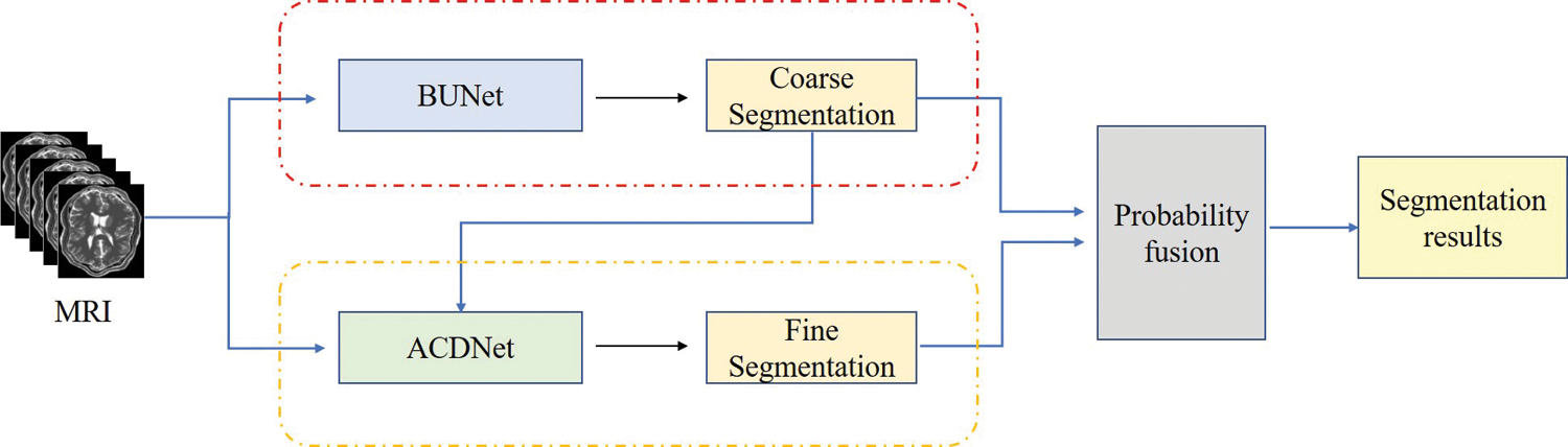
Figure 1: The proposed segmentation framework using cascaded network

3.2 Multi-Scale Feature for ACDNet

Multi-scale features have been widely used in image classification and segmentation. Its function is to fuse multi-scale information, increase the network receptive field and reduce the computation of network [22]. Especially in medical images with imbalanced categories, fusing multi-scale features is an important method to improve image segmentation performance. DenseNet uses cross-layer connections to make full use of features, and uses dense block between different layers to enhance feature propagation and feature reuse, which helps to alleviate the problem of gradient disappearance. Atrous Spatial Pyramid Pooling [23] (ASPP) was proposed in in Deeplab v3 [21]. Its principle is to obtain multi-scale information at different scales with different hole rates. Each scale is an independent branch. The network combines the features of different scales and adds a convolutional layer to output prediction labels.

In this work, the second layer added an ASPP module before the Bottle Neck layer of each block to assist in extracting multi-scale feature information. The bottle neck layer is a 1×1 convolutional layer, which was used to provide feature compression. When training, each block was used as a small network, and each block was set with a convolutional layer, a BN layer and a ReLU layer. The structure of each block was consistent, and the use of dense connections between blocks could be stacked, which made the network structure easier to adjust [24]. The structure of ACDNet is shown in Fig. 2.

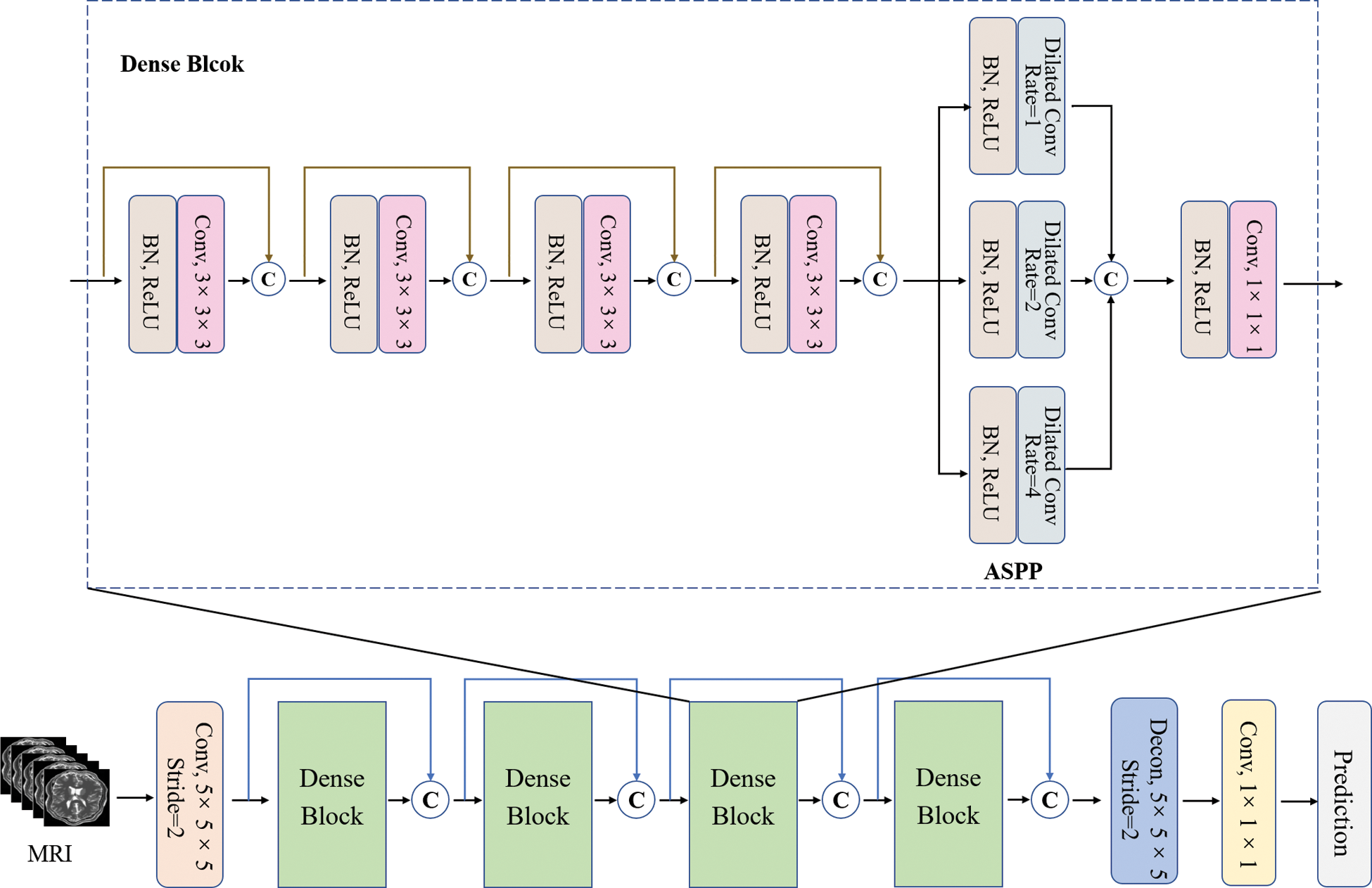
Figure 2: Structure of ACDNet

The deeper the network is, the more likely it is to have the gradient disappearance problem. Dense connection can be described that each layer is directly connected to the Input and Loss. It can alleviate the gradient disappearance problem and enhance the reuse of features, so that it can improve the accuracy of the segmentation.

3.3 Loss Metrics

There is a serious class imbalance problem in medical images [25]. In the NPC image segmentation task, because the background samples are relatively large, the network tends to predict the background, but the target is not completely predicted. Therefore, it is necessary to modify Cross Entropy (CE) of the loss function to reduce the weight of the background samples. Weighted cross entropy adds weights to different categories, so that the network pays attention to the categories with fewer samples. A coefficient is used to describe the importance of samples in the loss function. For a small number of samples, its contribution to the loss function should be enhanced; but for a large number of samples, its contribution to the loss function should be reduced.

In general, the “hard” samples are distributed along the segmentation boundary, with a probability of 0.5 in the probability response graph. Focal Loss [26] is a weighted cross entropy. This loss function reduces the weight of many simple negative samples in training, solves the problem of class imbalance, and helps to mine “hard” samples.

In the binary classification task, the cross entropy of loss function is defined as:

CE(p,y)={−log⁡(p),y=1−log⁡(1−p),otherwise (1)

The predicted probability value of category t can be expressed as:

pt={py=11−potherwise (2)

Substituting Eq. (2) into Eq. (1), we can get:

CE(p,y)=CE(pt)=−log⁡(pt) (3)

When many simple samples are added together, small loss values can dominate the rare categories. Therefore, the weight parameter α∈ [0,1] is used to adjust the CE value when the category is unbalanced. The equation is as follows:

CE(pt)=−αtlog⁡(pt) (4)

In Eq. (4), a weight parameter αt is added when loss is calculated for different categories. If the weight of categories with few samples is higher, the network prediction effect can be improved. However, Eq. (4) only solves the problem of weight distribution of different categories. For “hard” samples with a probability of about 0.5, the network still cannot segment these voxel points. Focal loss uses the modulation factor (1−pt)γ to solve the problem of difficult sample mining. The equation is as follows:

FL(pt)=−(1−pt)γlog⁡(pt) (5)

where γ is a parameter that can be adjusted, γ >0. When a sample is predicted incorrectly, the probability pt is very small, and the modulation factor (1−pt)γ γ is close to 1, then the sample’s contribution to loss will not be penalized. On the contrary, if the sample prediction is successful and the probability pt is close to 1, then the weight of the well-divided sample is lowered and the sample’s contribution to loss is small.

The class imbalance and “hard” sample problems in medical images are both prominent, and combined with Eqs. (4) and (5), the final Focal loss formula is formed:

FL(pt)=−αt(1−pt)γlog⁡(pt) (6)

In this paper, the loss function is Focal Loss weighted tumor voxel distance. The distance from each voxel to the tumor boundary was taken as the weight parameter αt , and each voxel in the loss function had an independent weight. In the experiment, a distance map was calculated based on the real image value, and each voxel in the distance map represented the distance from the voxel to the tumor boundary. The weighted value only affected the tumor voxels and did not affect the non-tumor voxels. The distance calculation can be regarded as:

α={d(v,edge)+1in1out (7)

where d is the distance from the voxel to the tumor boundary. Inside the tumor, the minimum distance between the voxel and the tumor boundary is not less than 1, while the voxel outside the tumor area is always 1. The distance weights on both sides of the tumor boundary are very similar. For voxels at the tumor boundary, the penalty for predicting a positive sample was much greater than for predicting a negative sample. As a result, the network avoided this penalty by predicting nothing, which could reduce the total loss. Inside the tumor, if the tumor voxel was predicted as a non-tumor voxel, a greater penalty would be produced. The distance weight matrix was used to punish the error of the model on the boundary, which aimed to improve the extraction of tumor boundary with loss penalty.

4  Experiments and Results

4.1 Dataset and Pre-Processing

This experiment had been conducted using three-dimensional MRI images of 120 patients with NPC, which were from the same hospital. They were scanned by T1 High Resolution Isotropic Volume Examination (THRIVE [27]), which could obtain more obvious MRI tumor images than other MRI. The images have a voxel size of 0.6 × 0.6 × 3.0 mm3 . They were needed to pre-process the original image. Firstly, we cropped the original image to retain only the head image of the nasopharyngeal tumor at the neck and above, because the acquisition range of the original image was large but the position of the nasopharyngeal tumor in the image was relatively fixed. Secondly, the images were resampled to the voxel size of 1 × 1 × 1 mm3 . Thirdly, we used the up-down jitter method to crop the image in the Z direction, and used the greedy algorithm to remove the black area in the X and Y directions. The final image size was 160 × 198 × 103. Finally, in order to make full use of the limited data set, the center of each image was randomly selected for image block sampling, and the horizontal flip was used for data augmentation. Due to the random cropping, when the number of image blocks was increased enough, the neighborhood of each pixel including the image boundary might be selected multiple times. It was more conducive to the training and learning of the network. Fig. 3 shows three views of NPC images NPC images after being cropped.

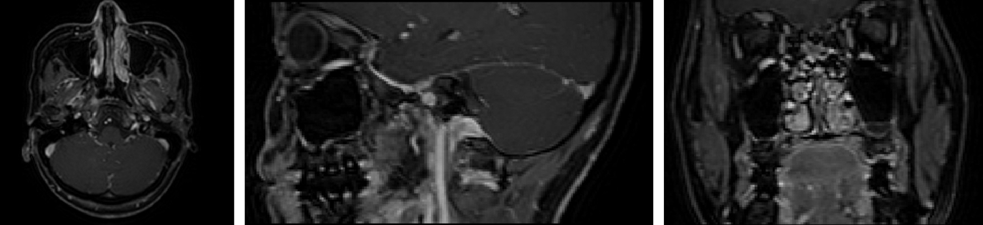
Figure 3: Three views of NPC images (Left: top view; Middle: lateral view; Right: front view)

4.2 Training Details

In the experiment, there were four automatic segmentation networks for comparison, including CNN, ACDNet, DeepLab and V-Net [28]. They were all the commonly used automatic segmentation networks. In order to obtain sufficient training samples, the images were sampled as an image block and input into the network for training. The image blocks were extracted as a training set by sliding window from the axial, coronal and sagittal directions of 3D MRI data respectively. Its size was 24 × 24 × 8.

Cross-validation was performed 5 times in the experiment. And in each cross-validation training, we randomly selected 24 patients’ images as the test set, 9 patients’ images as the validation set and 87 patients’ images as the training set. Predictions for 120 patients were obtained after 5 trainings. Fig. 4 shows the training accuracy curve, and Fig. 5 shows the loss function with distance weight.

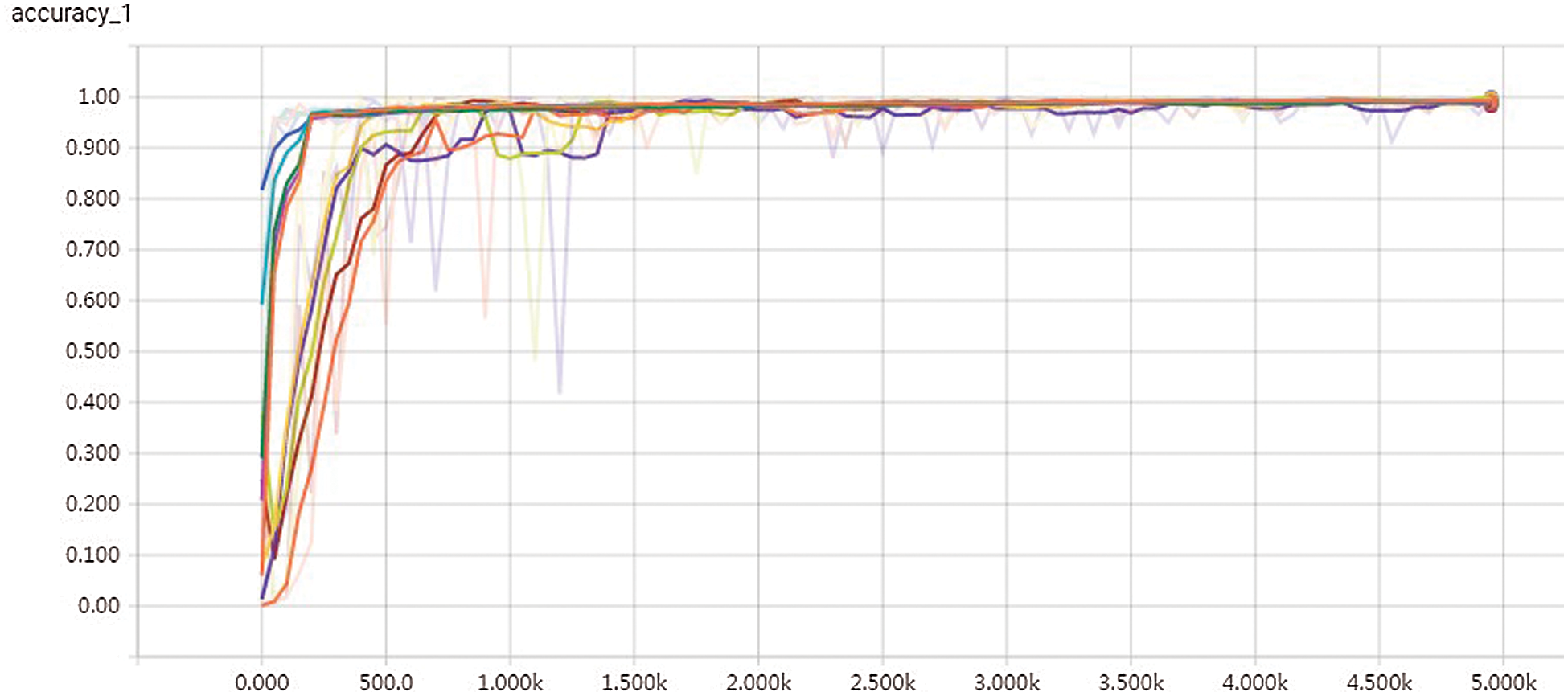
Figure 4: Training accuracy curve

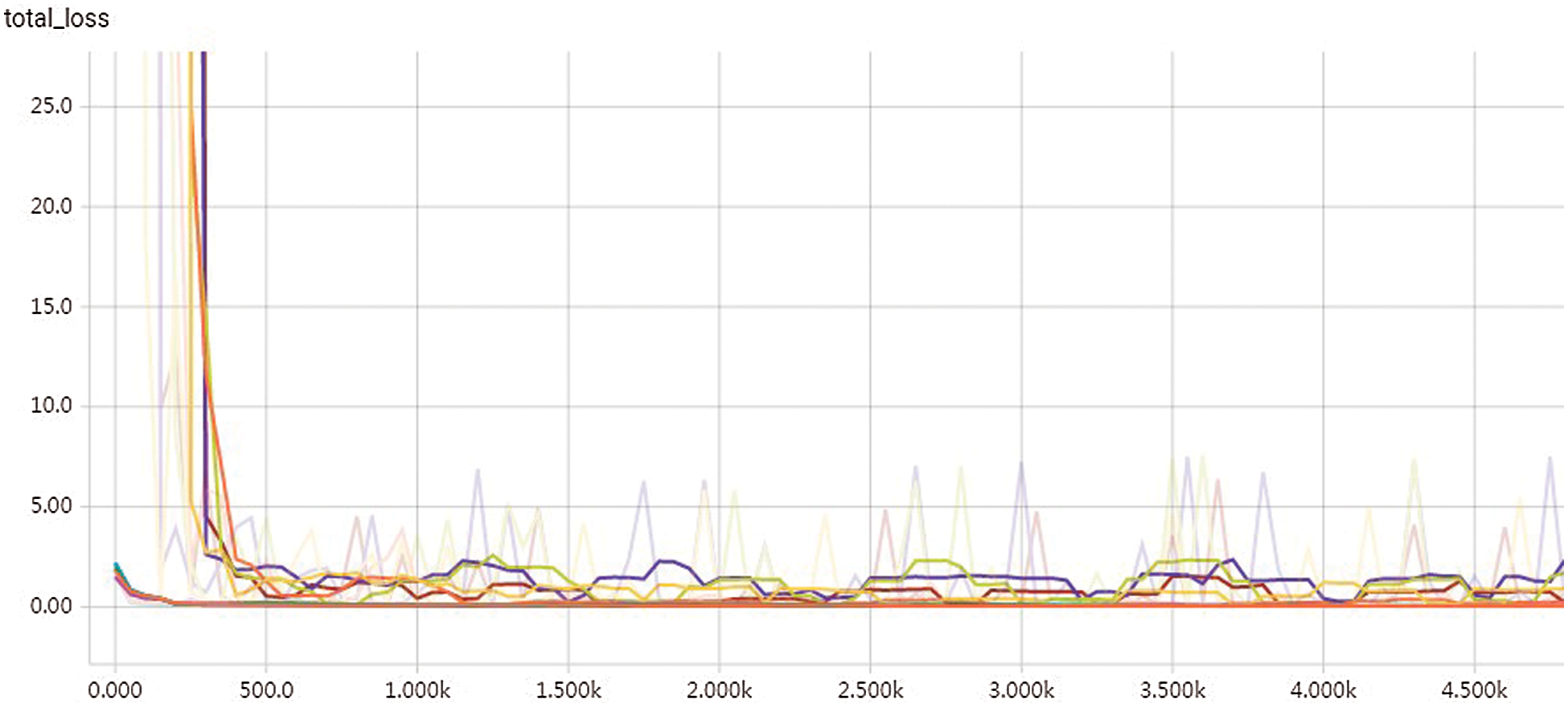
Figure 5: Loss function graph with distance weight

When training the network, we used the Adam optimizer and set the initial learning rate as 0.001. In all experiments, the number of training iterations was 50000, and the initial learning rate decreased exponentially with a decay rate of 0.9 per 500 iterations. All network structures used Softmax as the activation function to output the probability of the final split graph. Fig. 6 shows the curve of learning rate.

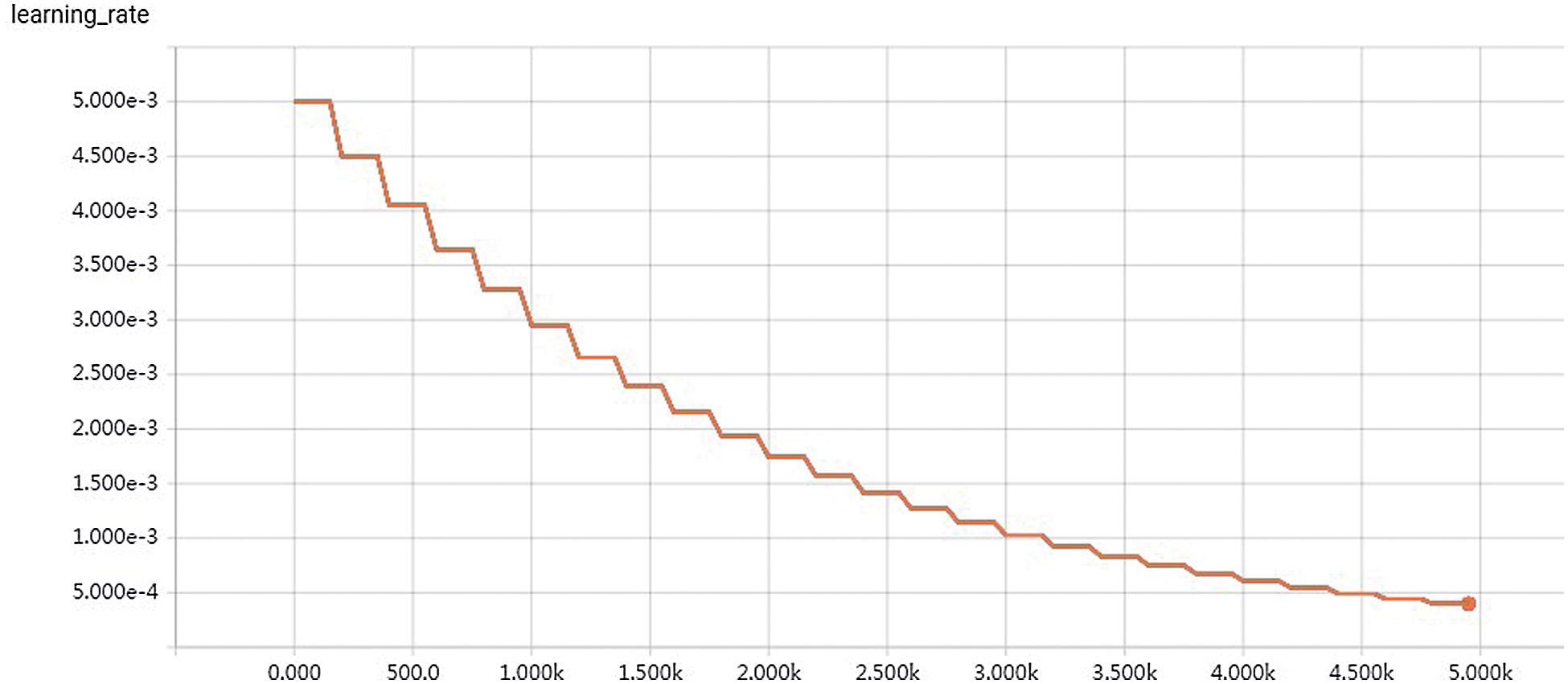
Figure 6: Curve of learning rate

4.3 Evaluation Metrics

There were three quantitative indicators to evaluate the segmentation performance of the network, including Dice Similarity Coefficient (DSC), Average Symmetric Surface Distance (ASSD) and F1-score.

DSC was used to measure the similarity between the segmentation results and the ground-truth [29]. For the given manually labeled tumor segmentation result X and predicted result Y of network segmentation, DSC is defined as:

DSC=2×|X∩Y||X|+|Y| (8)

where, |X∩Y| are the intersection between the labeled segmentation result and predicted result, |X| and |Y| represent the number of elements of X and Y. The value range of DSC is [0,1]. If the value of DSC is larger, the similarity between the network segmentation result and the real result is higher.

The ASSD index represents the average surface distance between the predicted results of network segmentation and the results of manual labeling segmentation. Its formula is as follows:

ASSD=12(∑g∈G⁡minp∈Pd(g,p)|G|+∑p∈P⁡ming∈Gd(p,g)|P|) (9)

where G and P represent the surface voxels of ground-truth and network prediction segmentation results respectively, and d(p,g) represents the Euclides distance between g and p .

F1-score was used to quantitatively evaluate the accuracy of network segmentation. It can be regarded as a weighted average of precision and recall. It is defined as follows:

F1_score=2×PRP+R (10)

where, the Precision is:

P=TPTP+FP (11)

where, the Recall rate is:

R=TPTP+FN (12)

where, TP is the true positive sample set, indicating the number of samples whose actual and predicted values are positive, that is, the predicted answer is correct. FP is the false positive sample set, representing the number of samples that are actually negative but predicted to be positive. FN is also the false negative sample set, which represents the number of samples that are actually positive but predicted to be negative. FP and FN both mean that the prediction is wrong. Precision represents the model’s ability to distinguish between negative samples. The higher the precision, the stronger the model’s ability to distinguish between negative samples. Recall rate reflects the model’s ability to identify positive samples. The higher the recall rate, the stronger the model’s ability to identify positive samples. F1-score takes into account both the precision and recall of the classification model. The larger the F1-score value is, the better the segmentation effect is, indicating that the model is more robust.

4.4 Results

The experimental results were evaluated qualitatively and quantitatively. Fig. 7 shows the two-dimensional segmentation results of different network structures on the same dataset in the experiment. Each row is the segmentation result of the same patient, showing 3 patients in total. Fig. 8 shows the 3D segmentation results of different network structures on the same dataset. It shows the coronal, sagittal, and axial segmentation results for the same patient.

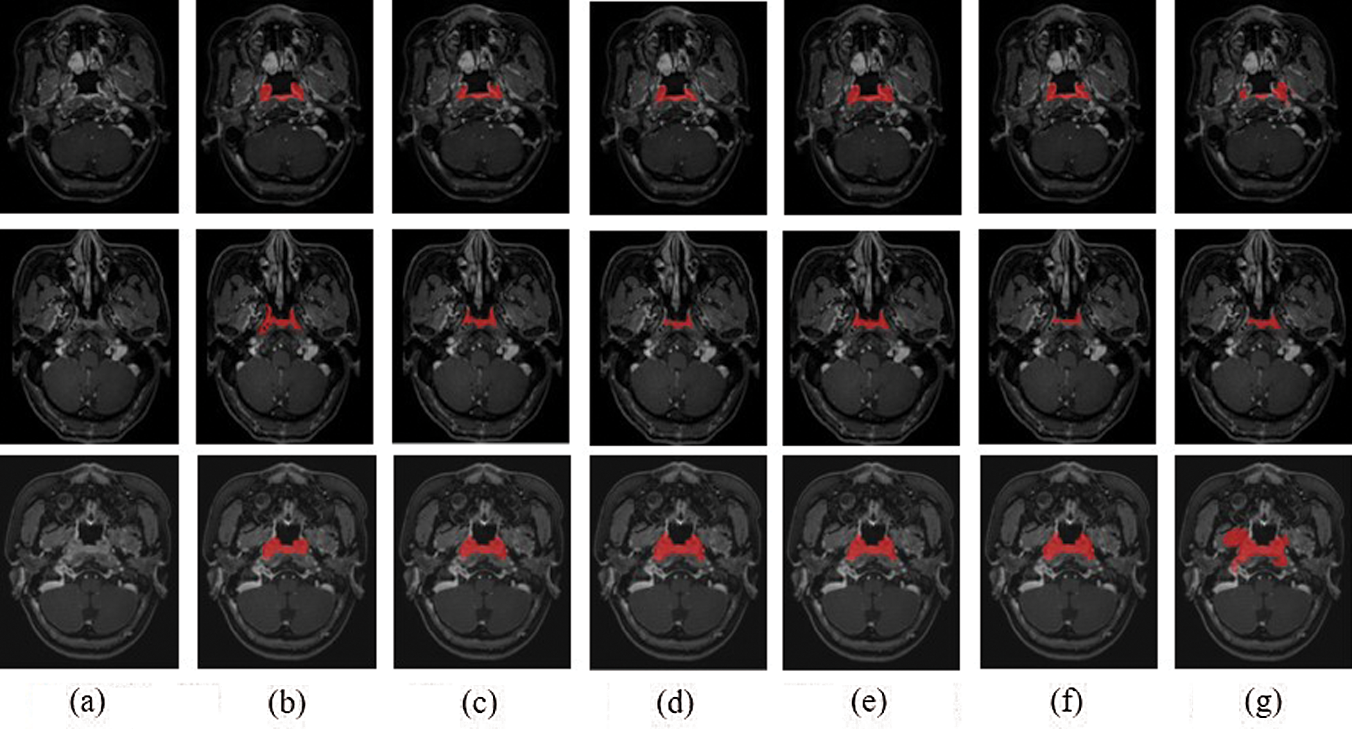
Figure 7: 2D segmentation graphs of different network structures on the same dataset (a) Raw (b) Ground truth (c) CSCN (d) CNN (e) ACDNet (f) Deeplab (g) V-Net

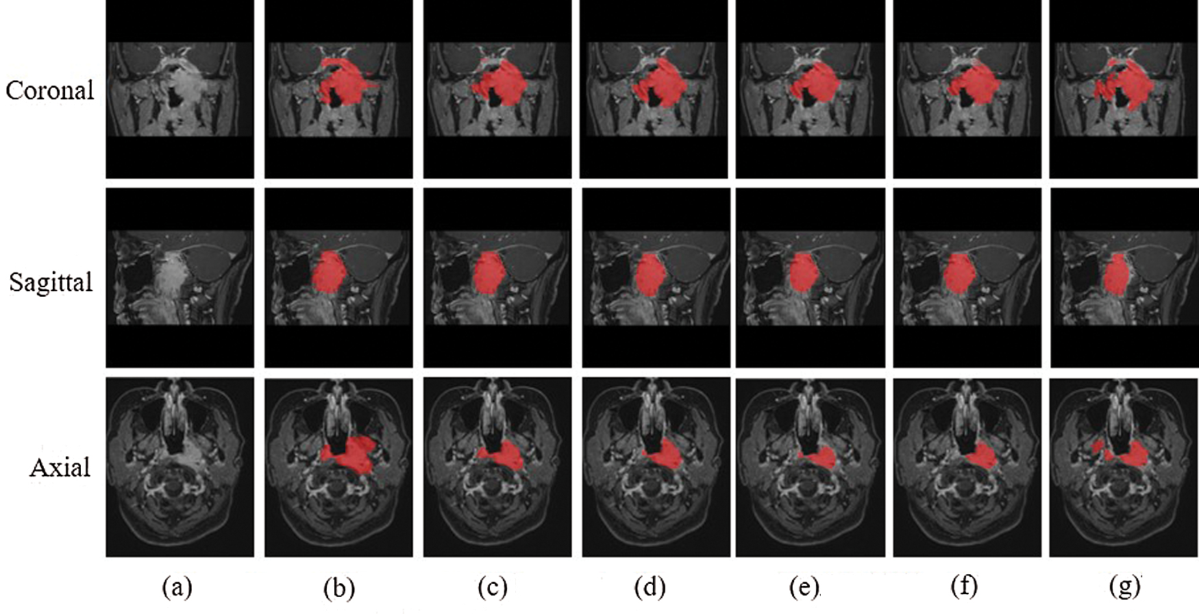
Figure 8: 3D segmentation graphs of different network structures on the same dataset (a) Raw (b) Ground truth (c) CSCN (d) CNN (e) ACDNet (f) Deeplab (g) V-Net

It can be seen from the figure that the segmentation effect of V-Net is not good. Its segmentation result is quite different from the Ground truth, which is not suitable for the segmentation of NPC images. The sagittal segmentation results of various methods are good, which are close to the Ground truth. In the coronal and axial segmentation, the method presented in this paper has the best performance.

Tab. 1 shows the quantitative evaluation values of various method, including DSC, ASSD and F1-score. It can be seen that CSCN has the best evaluation value. Compared with other networks, V-Net always failed to converge and the prediction result could not be obtained. In order to verify the performance of the algorithm, we used the annotation data of two physicians to compare. Each person annotated 28 patients’ MRI images, one of which was used as the Ground truth and the other as the prediction result. The values of DSC, ASSD and F1-score of the segmentation results were 0.642, 2.692 mm and 0.686 respectively.

5  Discussion and Conclusion

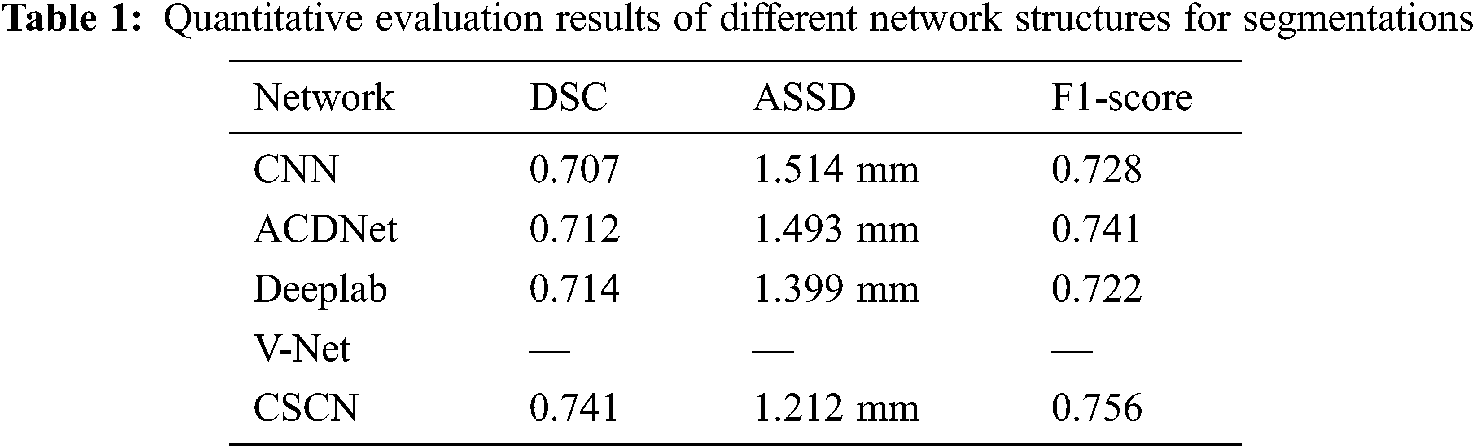
On the whole, the proposed network is superior to the contrast network in segmentation results and network performance. But for DSC, which values of manual labeling and network prediction segmentation results of doctors are not very good. In our analysis, it was believed that the complex anatomical structure of nasopharynx and slight surface differences caused by some tumors with special shapes would have a great impact on DSC indicators.

In this work, we proposed a coarse-to-fine cascaded fully convolutional network segmentation method. This algorithm used cascaded network and multi-scale feature skip connection to improve the segmentation effect. In the first network, random sampling was carried out from the axial, coronal and sagittal directions respectively to alleviate the problem of image category imbalance and the shortage of training samples. The tumor probability map of coarse segmentation was obtained, which was regarded as the input for the second network. In the second network, Atrous Spatial Pyramid Pooling was used to replace the convolution layer and pooling layer in the Dense block of DenseNet, so that multi-scale features were extracted to achieve voxel-level fine segmentation of MRI images. The cascaded network can alleviate the problem of gradient disappearance and obtain a smoother boundary.

Acknowledgement: The authors would like to thank all participants for their valuable discussions regarding the content of this article.

Funding Statement: This work was supported by the National Natural Science Foundation of China (Grant No. 81901828), the Sichuan Science and Technology program (Grant No. 2019JDJQ0002) and the Education Department Foundation of Chongqing (Grant No. 19ZB0257).

Conflicts of Interest: The authors declare that they have no conflicts of interest to report regarding this study.

References

 1.  M. F. Ji, W. Sheng, W. M. Cheng, M. H. Ng, B. H. Wu et al., “Incidence and mortality of nasopharyngeal carcinoma: Interim analysis of a cluster randomized controlled screening trial (PRO-NPC-001) in southern China,” Annals of Oncology, vol. 30, no. 10, pp. 1630–1637, 2019. [Google Scholar]

 2.  H. Peng, R. Guo, L. Chen, Y. Zhang, W. F. Li et al., “Prognostic impact of plasma Epstein-Barr virus DNA in patients with nasopharyngeal carcinoma treated using Intensity-Modulated Radiation Therapy,” Scientific Reports, vol. 6, pp. 1–9, 2016. [Google Scholar]

 3.  T. S. Hong, W. A. Tomé and P. M. Harari, “Heterogeneity in head and neck IMRT target design and clinical practice,” Radiotherapy and Oncology, vol. 103, no. 1, pp. 92–98, 2012. [Google Scholar]

 4.  R. A. Naqvi, D. Hussain and W. Loh, “Artificial intelligence-based semantic segmentation of ocular regions for biometrics and healthcare applications,” Computers, Materials & Continua, vol. 66, no. 1, pp. 715–732, 2021. [Google Scholar]

 5.  D. D. Patil and S. G. Deore, “Medical image segmentation: A review,” International Journal of Computer Science and Mobile Computing, vol. 2, no. 1, pp. 22–27, 2013. [Google Scholar]

 6.  H. Peng and Q. Li, “Research on the automatic extraction method of web data objects based on deep learning,” Intelligent Automation & Soft Computing, vol. 26, no. 3, pp. 609–616, 2020. [Google Scholar]

 7.  M. Radhakrishnan, A. Panneerselvam and N. Nachimuthu, “Canny edge detection model in MRI image segmentation using optimized parameter tuning method,” Intelligent Automation & Soft Computing, vol. 26, no. 6, pp. 1185–1199, 2020. [Google Scholar]

 8.  O. Ronneberger, P. Fischer and T. Brox, “U-Net: convolutional networks for biomedical image segmentation,” in Proc. of the Int. Conf. on Medical Image Computing and Computer-assisted Intervention (MICCAIMunich, Germany, pp. 234–241, 2015. [Google Scholar]

 9.  F. Guo, C. H. Shi, X. J. Li, X. Wu, J. L. Zhou et al., “Image segmentation of nasopharyngeal carcinoma using 3D CNN with long-range skip connection and multi-scale feature pyramid,” Soft Computing, vol. 24, no. 16, pp. 12671–12680, 2020. [Google Scholar]

10. G. Litjens, T. Kooi, B. E. Bejnordi, A. A. A. Setio, F. Ciompi et al., “A survey on deep learning in medical image analysis,” Medical Image Analysis, vol. 42, pp. 60–88, 2017. [Google Scholar]

11. S. Ghosh, N. Das, I. Das and U. Maulik, “Understanding deep learning techniques for image segmentation,” ACM Computing Surveys, vol. 52, no. 4, pp. 1–35, 2019. [Google Scholar]

12. C. Song, X. Cheng, Y. X. Gu, B. J. Chen and Z. J. Fu, “A review of object detectors in deep learning,” Journal on Artificial Intelligence, vol. 2, no. 2, pp. 59–77, 2020. [Google Scholar]

13. W. Fang, L. Pang and W. N. Yi, “Survey on the application of deep reinforcement learning in image processing,” Journal on Artificial Intelligence, vol. 2, no. 1, pp. 39–58, 2020. [Google Scholar]

14. S. A. Taghanaki, K. Abhishek, J. P. Cohen, J. Cohen-Adad and G. Hamarneh, “Deep semantic segmentation of natural and medical images: A review,” Artificial Intelligence Review, vol. 54, pp. 137–178, 2021. [Google Scholar]

15. X. D. Xue, X. Y. Hao, J. Shi, D. Yi, W. Wei et al., “Auto-segmentation of high-risk primary tumor gross target volume for the radiotherapy of nasopharyngeal carcinoma,” Journal of Image and Graphics, vol. 25, no. 10, pp. 2151–2158, 2020. [Google Scholar]

16. L. Lin, Q. Dou, Y. M. Jin, G. Q. Zhou, Y. Q. Tang et al., “Deep learning for automated contouring of primary tumor volumes by MRI for nasopharyngeal carcinoma,” Radiology, vol. 291, no. 3, pp. 677–686, 2019. [Google Scholar]

17. H. Chen, Y. X. Qi, Y. Yin, T. X. Li, X. Q. Liu et al., “MMFNet: A multi-modality MRI fusion network for segmentation of nasopharyngeal carcinoma,” Neurocomputing, vol. 394, no. 21, pp. 27–40, 2020. [Google Scholar]

18. S. H. Diao, J. X. Hou, H. Yu, X. Zhao, Y. K. Sun et al., “Computer-aided pathologic diagnosis of nasopharyngeal carcinoma based on deep learning,” American Journal of Pathology, vol. 190, no. 8, pp. 1691–1700, 2020. [Google Scholar]

19. G. Huang, Z. Liu, L. V. D. Maaten and K. Q. Weinberger, “Densely connected convolutional networks,” in Proc. of the IEEE Conf. on Computer Vision and Pattern Recognition (CVPRHonolulu, HI, USA, pp. 4700–4708, 2017. [Google Scholar]

20. Y. Sun, X. Wang and X. Tang, “Deep convolutional network cascade for facial point detection,” in Proc. of the IEEE Conf. on Computer Vision and Pattern Recognition (CVPRPortland, OR, USA, pp. 3476–3483, 2013. [Google Scholar]

21. L. C. Chen, G. Papandreou, F. Schroff and H. Adam, “Rethinking atrous convolution for semantic image segmentation,” in Proc. of the IEEE Conf. on Computer Vision and Pattern Recognition (CVPRHawaii, USA, 2017. [Online]. Available: arXiv: 1706.05587. [Google Scholar]

22. D. G. Shen, G. R. Wu and H. Suk, “Deep learning in medical image analysis,” Annual Review of Biomedical Engineering, vol. 19, pp. 221–248, 2017. [Google Scholar]

23. L. C. Chen, Y. K. Zhu, G. Papanreou, F. Schroff and H. Adam, “Encoder-decoder with atrous separable convolution for semantic image segmentation,” in Proc. of the European Conf. on Computer Vision, Munich, Germany, pp. 833–851, 2018. [Google Scholar]

24. L. R. Bonta and N. U. Kiran, “Efficient segmentation of medical images using dilated residual network,” Computer Aided Intervention and Diagnostics in Clinical and Medical Images, vol. 31, pp. 39–47, 2019. [Google Scholar]

25. C. Luo, C. H. Shi, X. J. Li, X. Wang, Y. C. Chen et al., “Multi-task learning using attention-based convolutional encoder-decoder for dilated cardiomyopathy CMR segmentation and classification,” Computers, Materials & Continua, vol. 63, no. 2, pp. 995–1012, 2020. [Google Scholar]

26. T. Y. Lin, P. Goyal, R. Girshick, K. M. He and P. Dollár, “Focal loss for dense object detection,” in Proc. of the IEEE Int. Conf. on Computer Vision (ICCVVenice, Italy, pp. 2999–3007, 2017. [Google Scholar]

27. L. I. Baocan, F. Kong, W. Huang and M. Center, “The value of enhanced T1 high resolution isotropic volume examination (eTHRIVE) on evaluation of collateral vessels in esophageal gastric varices,” Journal of Clinical Radiology, vol. 32, no. 9, pp. 1300–1304, 2013. [Google Scholar]

28. F. Milletari, N. Navab and S. A. Ahmadi, “V-Net: Fully convolutional neural networks for volumetric medical image segmentation,” in Proc. of the Fourth Int. Conf. on 3D Vision (3DVStanford, CA, USA, vol.1, pp. 565–571, 2016. [Google Scholar]

29. K. H. Zou, S. K. Warfield, A. Bharatha, C. M. C. Tempany, M. R. Kaus et al., “Statistical validation of image segmentation quality based on a spatial overlap index1: Scientific reports,” Academic Radiology, vol. 11, no. 2, pp. 178–189, 2004. [Google Scholar]

This work is licensed under a Creative Commons Attribution 4.0 International License, which permits unrestricted use, distribution, and reproduction in any medium, provided the original work is properly cited.