DOI:10.32604/iasc.2022.020560
| Intelligent Automation & Soft Computing DOI:10.32604/iasc.2022.020560 | |
| Article |
Application of Fuzzy FoPID Controller for Energy Reshaping in Grid Connected PV Inverters for Electric Vehicles
1Department of EEE, Mar Ephraem College of Engineering and Technology, Elavuvilai, Marthandam, 629171, India
2Department of EEE, Arunachala College of Engineering for Women, Manavilai, Vellichanthai, 629203, India
*Corresponding Author: M. Manjusha. Email: manjushaj6191@gmail.com
Received: 29 May 2021; Accepted: 16 July 2021
Abstract: By utilizing Fuzzy based FOPID-controller, this work is designed via the energy reshaping concept for Grid connected Photovoltaic (PV) systems for electric vehicles and this PV module has its own inverter which is synchorised with the utility grid. In grid connected PV system, the mitigation plays an important role where the capacity of PV arrays increases it maintains power quality and it is necessary to comply with some requirements such as harmonic mitigation. Unless a maximum power point tracking (MPPT) algorithm is used, PV systems do not continuously produce their theoretical optimal power. Under various atmospheric conditions, MPPT is obtained by using Perturb and Observe (P&O) techniques. A storage function in terms of DC-link voltage and current, and q-axis current is created, by means of which physical characteristics are studied. Further the energy reshaping is done with the aid of the proposed Fuzzy Fractional Order PID (Fuzzy-FoPID) framework. The FOPID control parameters λ and μ are optimally tuned by Grey Wolf Optimization technique (GWO). The results obtained verify the advantages of using Fuzzy-FoPID control as compared to conventional PID (Proportional Integral Derivative) control and FoPID control. The injected reactive power into the grid and the efficiency of the proposed systems is studied by extensive simulations.
Keywords: Current controller; voltage regulator; grid connected inverter; electric vehicles; PID controller
Among various types of renewable energy resources as per the abundance of renewable resources, simple installation of PV technologies, secure operation with low operating costs, PV schemes are getting enormous popularity [1].
Proportional resonant control have fulfilled steady-state efficiency, but any variation in the frequency of the grid can have adverse effects on its performance [2]. The most sophisticated controller for tracking repetitive periodic signals including sinusoidal waveforms is the repetitive controller. The design of the FLC (Fuzzy Logic Controller) is becoming easy, without in-depth knowledge of the system, for complex and nonlinear process. The adaptive nature by the fuzzy system enhances the FO controller’s dynamic output, through which the controller will respond quickly to the variation of parameters. so that improved control efficiency with simple physical understanding can be achieved [3]. GWO technique is employed to tune the parameters of PID controller of doubly-fed induction generator-based wind turbine [4]. This paper adopts GWO, which modifies the hierarchy of wolf hunting by introduction of further roles of wolf to achieve a balance between exploration and exploitation, and control parameters can be optimized by this algorithm.
Shun-Cheung wang et al. (2020) suggest a simple and efficient maximum power tracking method that combines simplified model-based state estimation (SMSE) with the adaptive alpha perturb-and- observe (P&O) method. Swati Singh et al. (2020) represented that review of optimization and modeling methodologies, as well as the interface mechanism of various renewable energy sources with various control designs such as the Fuzzy Controller, Fractional Order FPID (Fuzzy PID) Controller, and FOPID (Fractional Order PID) Controller. Majid Dehghani et al. (2021) presented that to achieve the full PowerPoint; a fuzzy logic controller (FLC) was optimized by a combination of particle swarm optimization (PSO) and genetic algorithm (GA).
Research Gap
As stated above, various control algorithms have been proposed to improve the efficiency and various energy reshaping [5] approaches have been used. But still there is a need for improvement in efficiency for use in practical applications, hence the research.
Contribution of the proposed research include
i. A novel energy reshaping approach using Fuzzy FOPID controller is proposed.
ii. The above strategy has been applied to a grid connected PV inverter.
iii. To obtain maximum solar energy from the PV array under various atmospheric conditions, MPPT technique is utilized.
iv.iv. The efficiency of the proposed approach is studied extensively and compared with the existing approaches available in the literatures.
2 Proposed Energy Reshaping Scheme for Grid Connected PV System
The proposed system is based on a grid-connected PV inverter with MPPT technology and the following converter descriptions and Fig. 1 are provided below. The inverter input is a DC source voltage or a rectifier output. The output is connected to the grid to transfer power [6] to the grid through a low-pass filter.
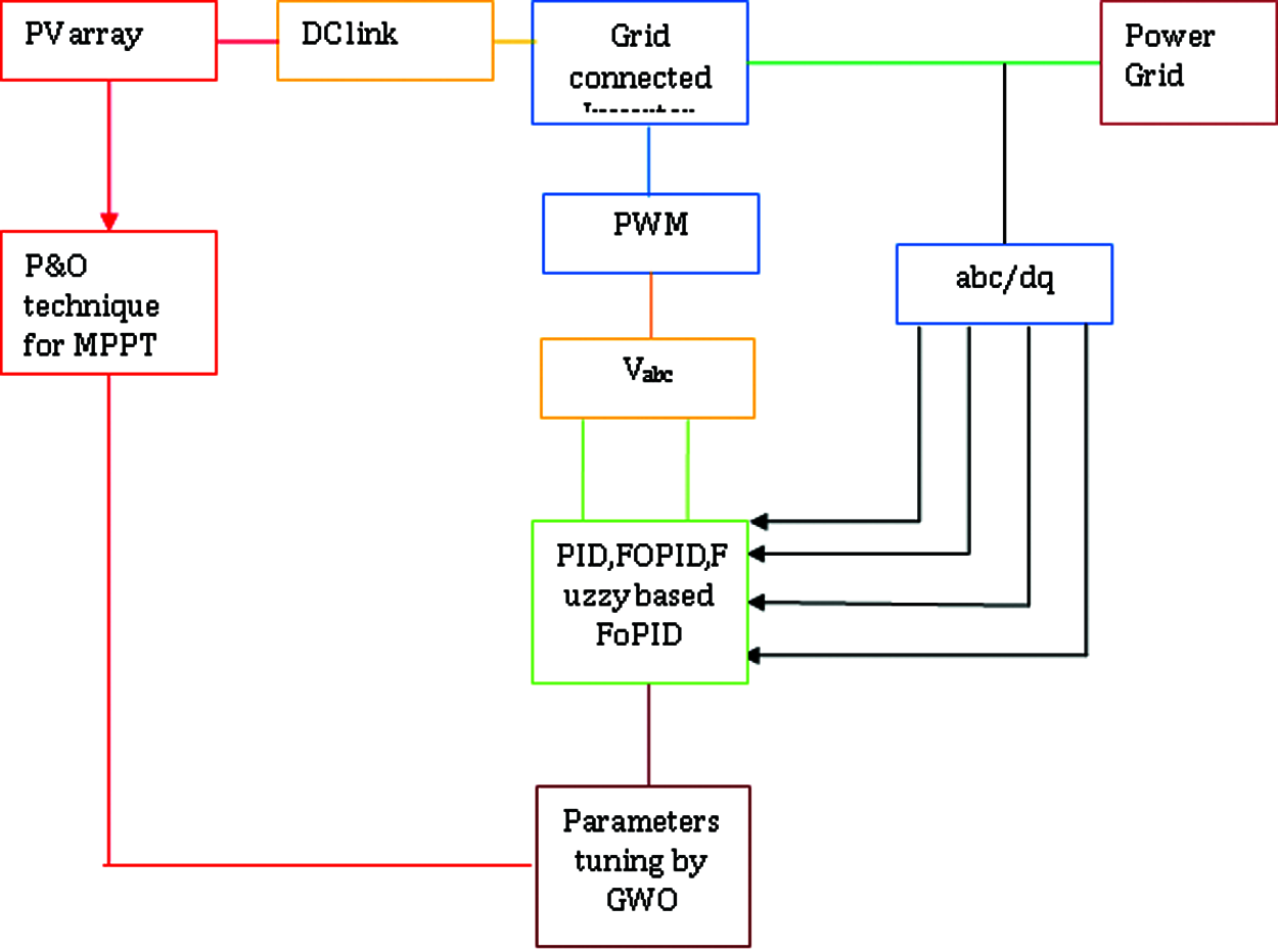
Figure 1: Block diagram of grid connected PV inverter with MPPT technique
With the interconnection of several PV modules a photovoltaic array is a simple serial and/or parallel. In general, the modules are initially connected in a serial [7] manner to obtain the required voltage, when constructing a PV array.
Mathematical modelling of PV panel: As irradiation is proportional to current, diode is connected in parallel with the current source in the recombination losses are represented. The equivalent circuit of a functional PV cell where the current is produced is shown in Fig. 2 and the V-I characteristics of the PV array in Fig. 3.
q –electron charge, Iph- photo electric current, n -No. of cells in series, T -Absolute temperature in Kelvin, Im - the current of module, k -Boltzmann constant, Ns, Np–PV cells in series & b parallel
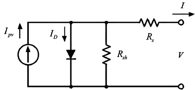
Figure 2: Equivalent circuit of the practical PV cell
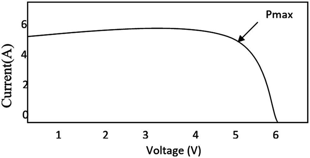
Figure 3: PV array V-I characteristics
Eq. (2) shows the relationship between the current and voltage output, where A is the p-n junction ideality factor, that ranges from1 to 5 and k, the Boltzman’s constant (1.3806* 10−23 J/K).
IPV - cell’s photo current, Is- Reverse saturation current of cell, Tc - Reference temperature of cell in K, q-electron charge in Cb, Vdc - PV output voltage.
The photo electric current as a function of the short circuit current is expressed as follows.
where Isco is the short circuit current at standard insolation G0(1000W/m2) and standard temperature T0(2510C), α is the module’s temperature coefficient for the current.
To get the MPP effectively under time-varying atmosphere P & O method is used. Temperature and power of the PV array (voltage and current), accurate monitoring of the MPP [8] is an essential factor in the model of effective solar [9] array systems [10].
P & O method: Variation in power is considered the major factor for MPPT in this process. Here, the successful perturbation in the duty cycle is in the same direction to hit the MPP on the rise in power, and would be in the opposite direction, on the decrease in power.
For the PV system in which a storage function associated DC-link current, DC-link voltage and q-axis current are constructed. Apply Kirchhoff’s current law, the dynamics [11] of the DC side is obtained as follows
C - DC bus capacitance
The three-phase two-level PV inverter dynamics in dq frame is given in the below equation
ed, eq, id, iq, vd and vq - dq-axis components of grid voltage, grid current, and PV inverter output voltage
R & L – resistance & inductance, ω -synchronous frequency of AC grid.
Assume the power loss in PV inverter switches are ignored, the power balance equation relating DC input and the AC output is given by
where Vdc and Idc - PV inverter input current and voltage state vector
x = (x1x2x3)T= (idiqVdc)T, output y = (y1,y2)T= (iq, Vdc)T and input u = (u1,u2)T = (vd, vq)T.
The state equation of PV inverter as in Eq. (5) and Eq. (7) is given as,
The tracking error e = (e1,e2)T=
The control input ‘u’ appears explicitly, as differentiate the tracking error e
where,
With
The storage function H(iq, Idc, Vdc) is given as as the sum of heat produced by q-axis current iq, DC-link voltage Vdc and DC-link current Idc.
The inverter connected to the grid transforms DC into AC suitable for injection into the grid, usually 120 V RMS at 60 Hz or 240 V RMS at 50 Hz. Inverters [12] connected to the grid are used between local electricity generators [13] and this three-phase grid-connected PV inverter [14] configuration is shown in Fig. 4.
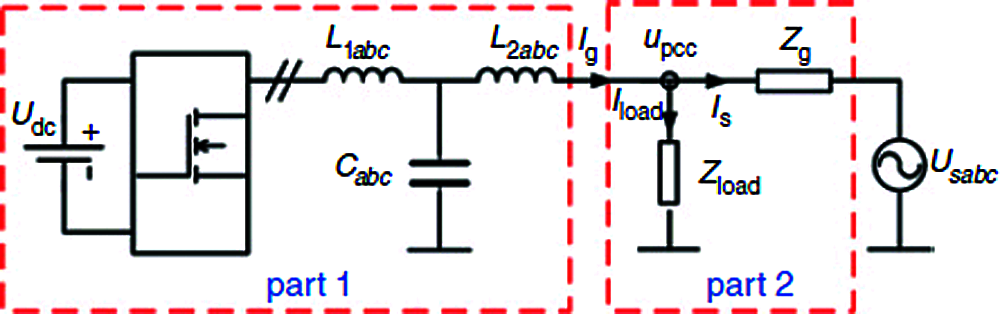
Figure 4: Three-phase grid-connected PV inverter configuration
The ideal voltage source [15] is in series with the grid impedance Zg. The grid current is expressed in Eq. (13), with an output impedance Zinv, the grid-connected inverter is considered a current source Icr in parallel. Zg(s)/Zinv(s) gives the grid-connected system Pm since under the assumption that current source Icr and the voltage source Us are independently stable.
The relative stability is proved, as the Pm of Zg(s)/Zinv(s) does not affect real Pm of the grid connected system although Icr is stable and the mathematical model of grid-connected inverter control system is shown in Fig. 5.
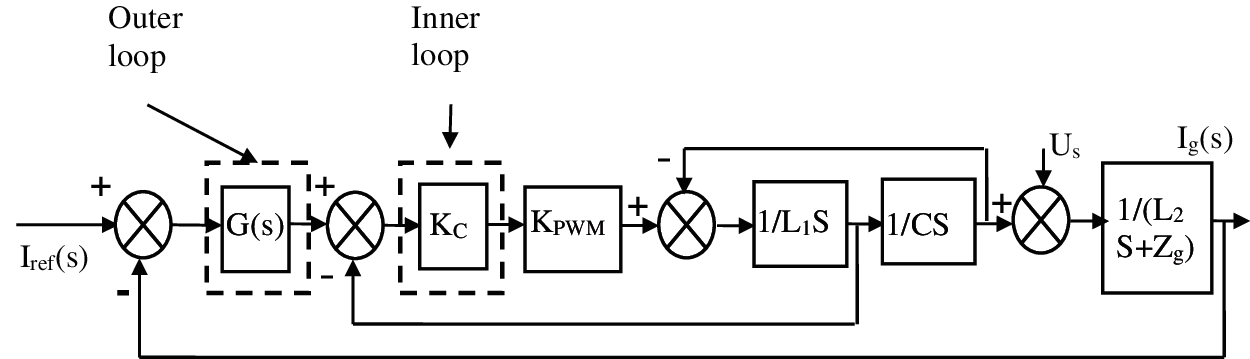
Figure 5: Mathematical model of grid-connected inverter control System
Provided that, according to Fig. 6, the inner loop is a proportional regulator Kc and outer most loop is a proportional-integral (PI) regulator. The transition function [16] of the closed loop is
Considering that Us is a perturbation, then Ig(s) can be rearranged as
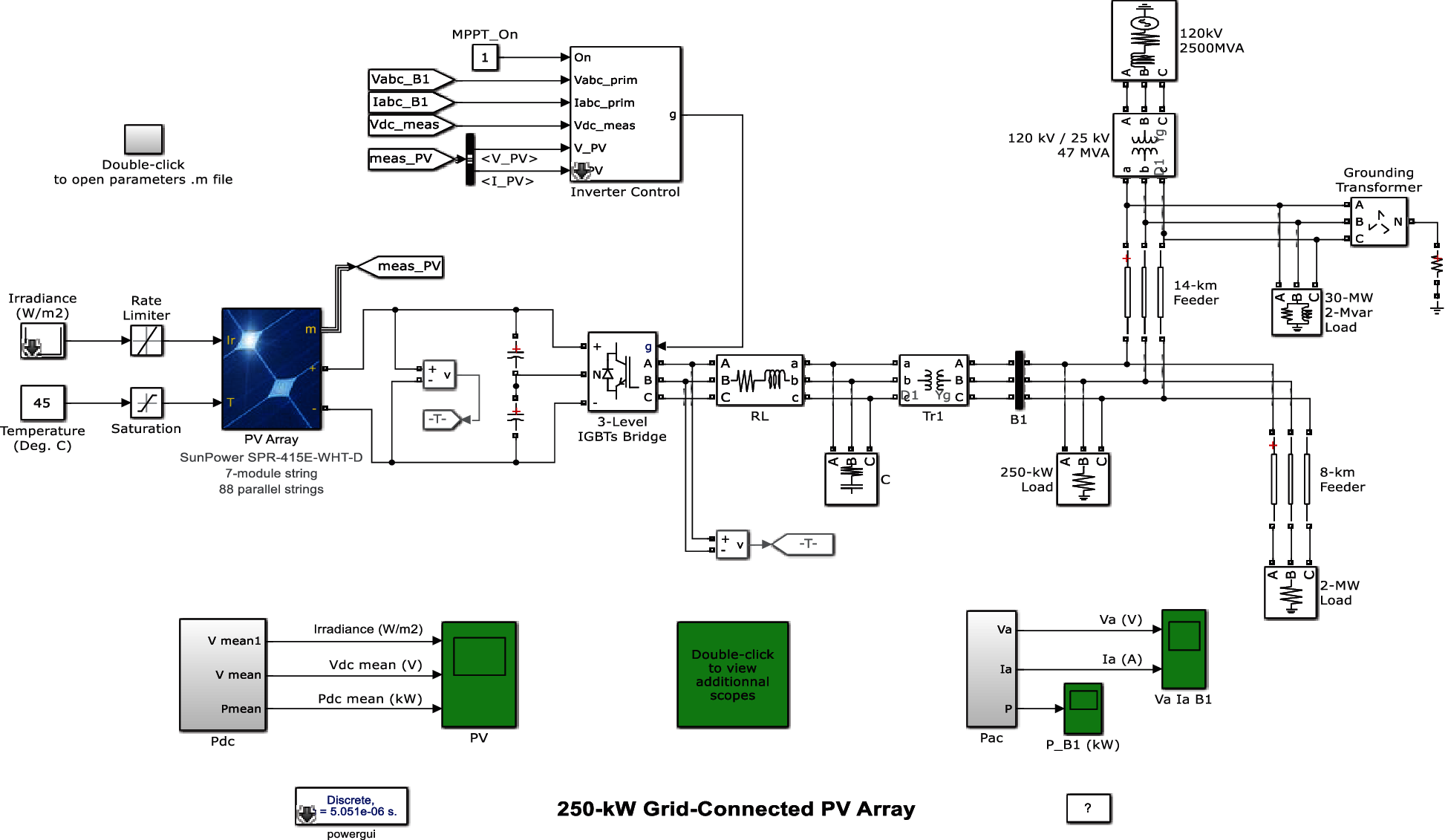
Figure 6: Simulink diagram of proposed Grid connected PV system
In Eq. (19), Zo(s) - sum of the inverter output impedance , Zinv(s) - grid impedance Zg(s). Moreover,
The coefficients of m1, m2 and m3 can be seen in Eq. (18). According to Eq. (13), it can be rearranged as
Calculated by the new mathematical model, comparing Eq. (22) with Eq. (19), Eq. (22) can be calculated as follows:
And Gclosed(s) is
3 Control Techniques and Energy Reshaping
The double loop control mode is adopted by a control system. The outer loop is used to manage the dc link voltage (V dc). The proportional integral (PI) controller is used to regulate the grid current and the dc-link voltage. The transfer function [17] of the PI controller looks like the following:
Kp = Proportional gain, Ki = Integral gain.
Proportional Control, the most important of these, calculates the extent of the difference between set point and process variable (known as error) and then makes sufficient proportional adjustments to the control variable to remove the error. The Control law for PID Controller [18] is
where
The fractional order controller (PID (λδ)) is the same as the traditional PID controller, but the only difference is the fractional derivative order (δ) and integral order (λ). The FoPID controller transfer function [19] illustration is given by,
where Gc(s) is controller transfer function, e(s) – error, c(s) – output. The term λ and μ are the fractional of integral [20] parts and derivative parts [21].
The time domain representation of FoPID controller is given in Fig. 9.
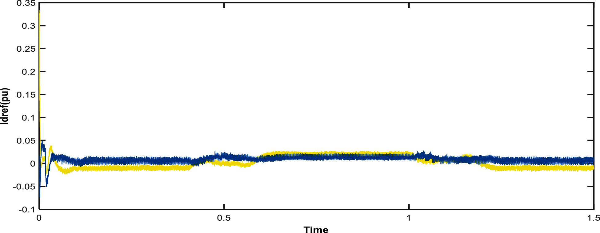
Figure 9: Current obtained with PI controller
3.4 Proposed Fuzzy FOPID Controller
The Fuzzy controller computes the scaling factor from error inputs to refresh the gain parameters of FOPID controller in an advanced systematic way.
where kp, kI, and kD - initial gains of FoPID and
Δkp, ΔkI, and ΔkD - scaling factors obtained from FLC.
For input and output fuzzy, triangle membership functions are used by applying Mamdani type inferencing system.
3.5 Proposed Fuzzy Based FOPID Control and Energy Reshaping
In the proposed method, FOPID attempts to designate a closed-loop energy feature which is analogous to the contrast between the system energy and the energy given by the controller. As follows, the energy modification equation is
where H(x) - storage function
From Eq. (12) the very first term of the storage function
Design Fuzzy based FoPID control for system,
The additional inputs υ1 and υ2 is designed in the fuzzy based FoPID control form, is as follows
As PID control gains KP1, KP2, KI1, KI2, KD1, KD2, fractional differentiator order μ1 and μ2, λ1 and λ2 are selected to achieve sufficient convergence of the tracking error.
3.6 Grey Wolf Optimization (GWO)
Grey wolf belongs to Canidae family. The pioneers also called as alpha are a male and female. The alpha is responsible for settling on decisions. The pack are directed by the decision taken by the alpha.
3.6.1 Steps to Find the Optimally Tuned Parameters of the Fuzzy Based FoPID Controller Using GWO Technique
In various design problems, GWO can fundamentally increase the global optimum and provide an efficient and viable instrument for controller tuning Encircling behavior is demonstrated by the following equations,
Hunting behaviour is described by following equations
where t indicates the current iteration,
Pseudo code of the GWO algorithm is presented below,
• Step 1: Initialize grey wolf population size Xi (i = 1, 2,3, …, n)
• Step 2: Initialize the parameters a, A, and C
• Step 3: Calculate fitness values of each search agent
Xα is best search agent
Xβ is second-best search agent
Xδ is third best search agent
• Step 4: Determine α, β and δ1
• Step 5:Update Hunting and Scouting
• Step 6: Fitness calculation of all search agents
The fitness value is measured at the kth and (k-1)th iteration, respectively as Fk and Fk−1.
• Step 7: Determine the α, β and δ1 based on the Fitness value
• Step 8: Update the position of the current search agent by equation
• Step 9: Update the parameters a, A, and C
• Step 10: Calculate fitness of entire search agent Fk − Fk−1 ≤ ε
Update the parameters Xα, Xβ, and Xδ
While k = k + 1; end; return Xα.
3.6.2 Optimal Parameter Tuning Using GWO Techniques
The Fuzzy based FoPID control parameters in Eq. (38) and Eq (39) are optimally tuned based on three cases, solar irradiation variation, temperature variation, and power grid voltage drop.
where the weights are ω1 and ω2.
4 Simulation Results and Discussion
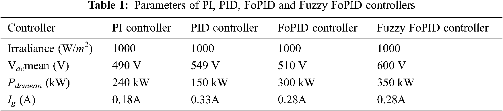
To improve the efficiency and robustness of PV power generation, proposed approach develops a specific model of grid-connected PV system by MATLAB/Simulink environment that accurately represents the system’s qualities. To figure the performance of proposed GWO based Meta heuristic MPPT algorithm, the performance was compared with PI controller, PID controller, FOPID controller and Fuzzy FoPID controller. The proposed Grid connected PV system Simulink chart is shown in Fig. 6 and Tab. 1 shows the parameters of PI, PID and FoPID controllers. Simulink graph of FOPID controller based current regulation is shown in Fig. 7 and Fig. 8 shows the simulink diagram of Fuzzy FoPI controller.
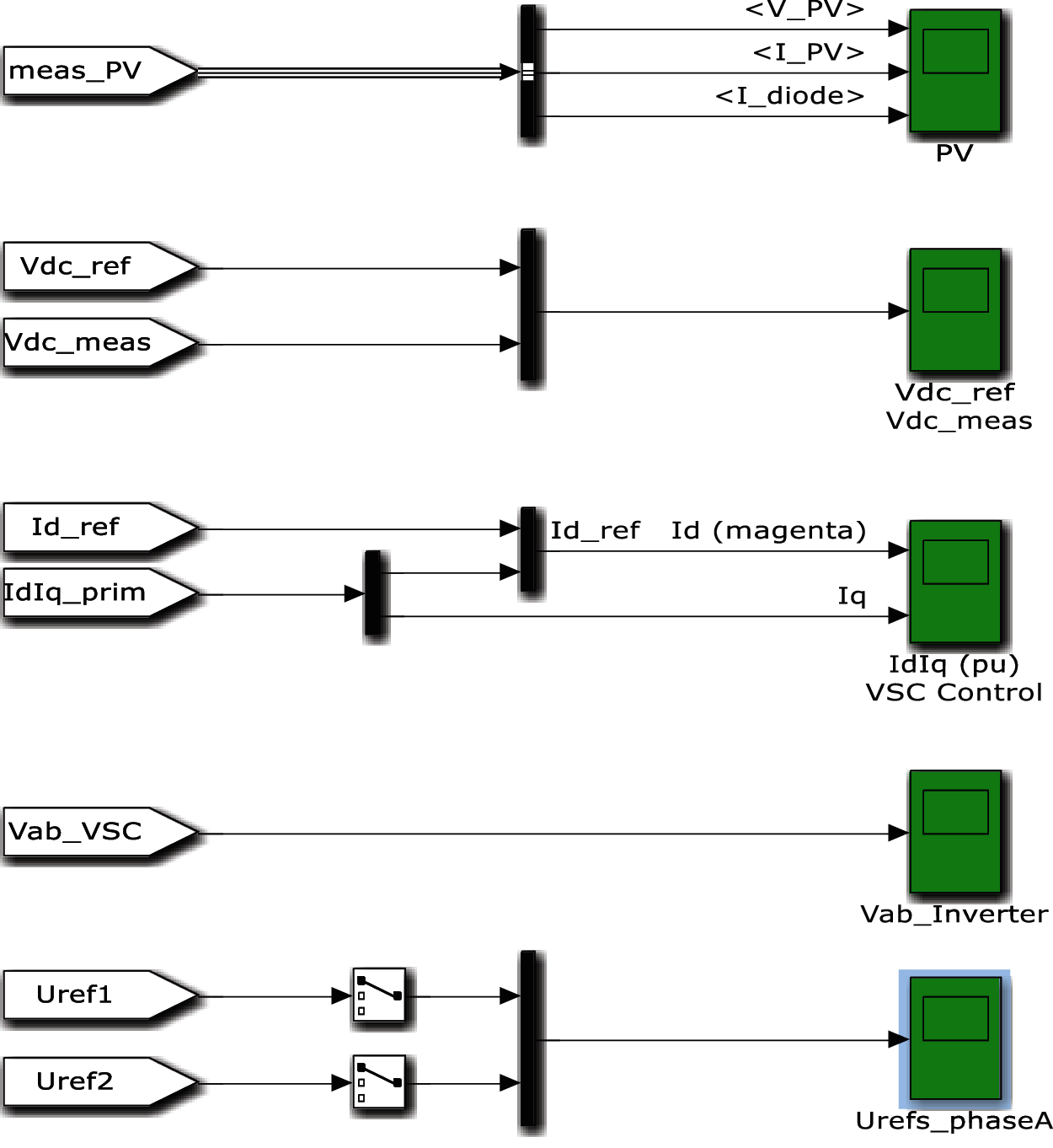
Figure 7: Simulink diagram of FOPID controller based current regulation

Figure 8: Simulink diagram of Fuzzy FoPI controller
From the outcomes, we can see that the output voltage of the PV panel settles down at 2 KV while the current worth changes depending on the irradiation. The Id reference esteem 0.03p.u which is given as the input sign of PI controller is shown in Fig. 9 and the Fig. 10 shows output voltage and current utilizing PI controller. As the output power used PI controller is shown in Fig. 11.
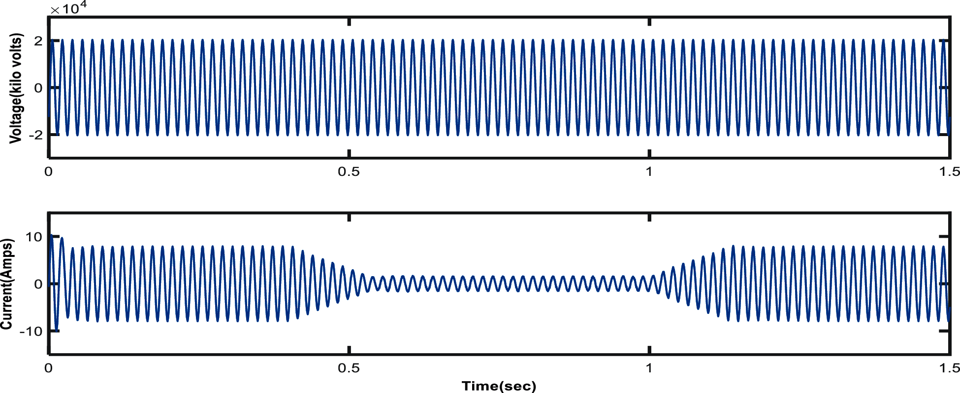
Figure 10: Output voltage and current using PI controller
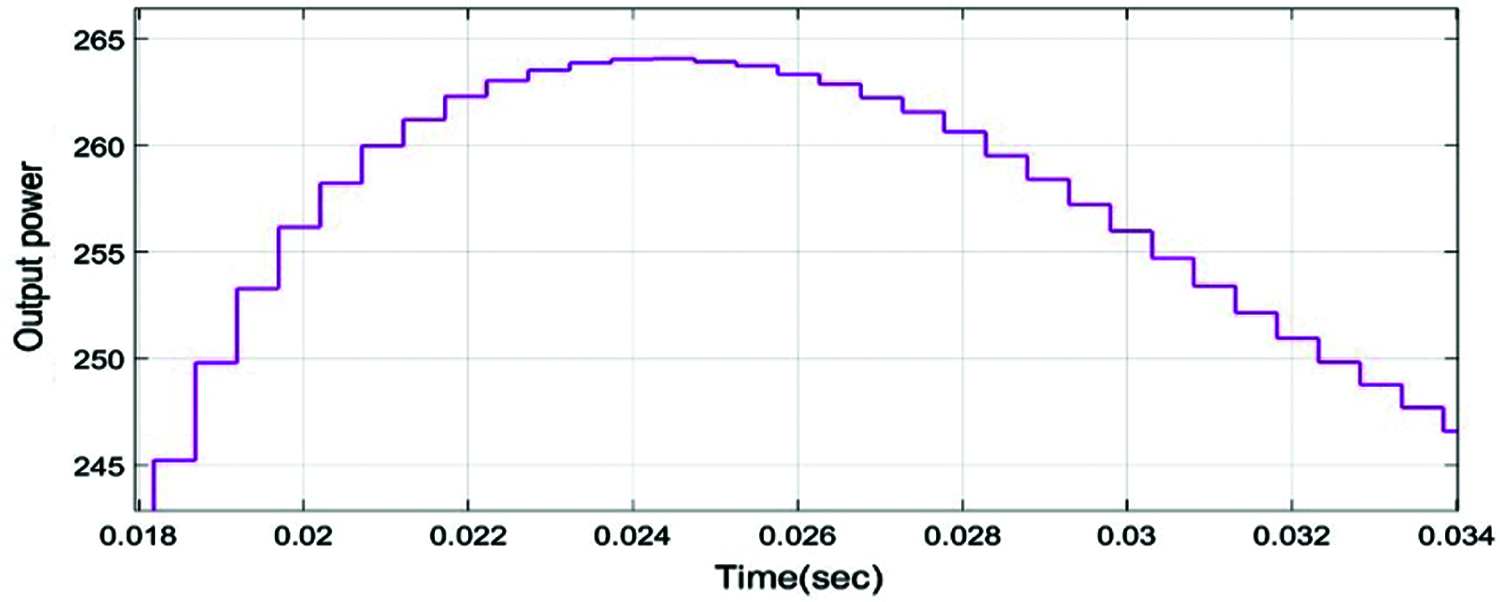
Figure 11: Output Power using PI controller
Sun irradiance is rapidly ramped down from 1000 W/m2 to 200 W/m2. Due to the MPPT operation, the control system lessens the VDC reference to 464 V to extricate maximum power from the PV cluster (46 kW). At t = 0.5 sec. At time t = 0.5 sec to t = 1sec, current decreases to 2A and so power drop occurs.
The irradiation esteems utilized in the simulations for example 800 W/m2 and 1000 W/m2 and its shown in Fig. 12. Fig. 12 shows the irradiance, Input dc voltage and input power of the PV panel. we get a PV voltage (Vdc mean) of 2 kV and the power removed (Pdc mean) from the exhibit is 150 kW When the consistent state is stretched (around t = 0.15 sec.). Fig. 13 shows the voltage and current wavefrm of PID controller and this PID controller output power is shown in Fig. 14.
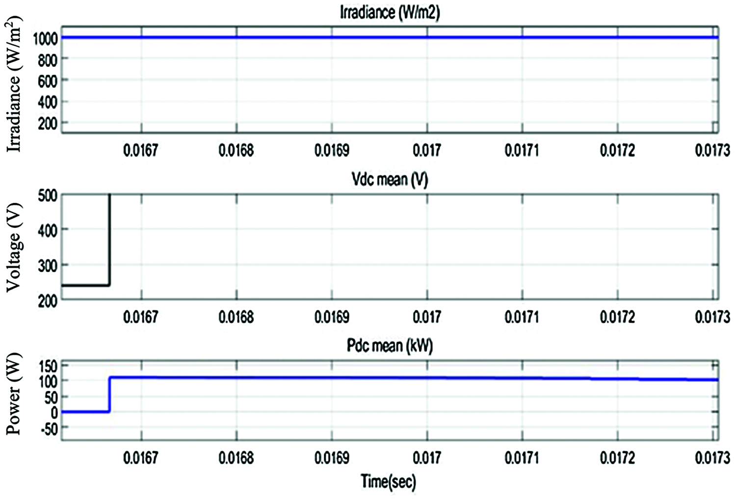
Figure 12: Irradiance, input dc voltage, input power of PV panel
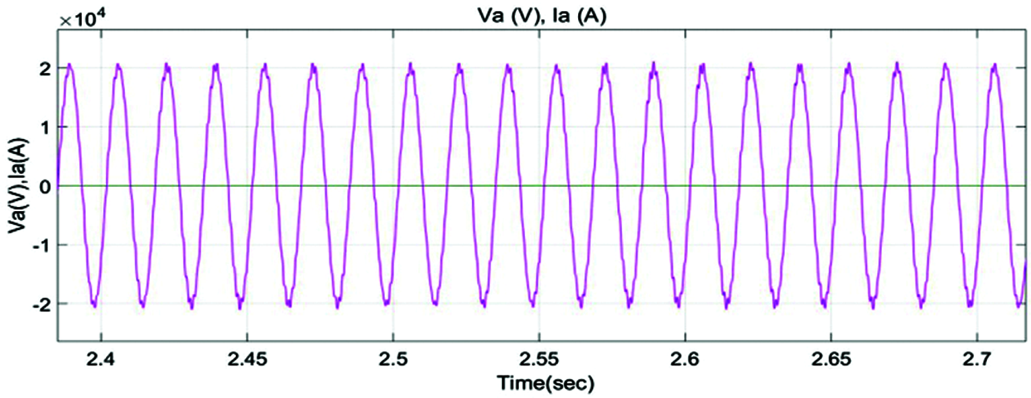
Figure 13: Current and voltage of converter with PID
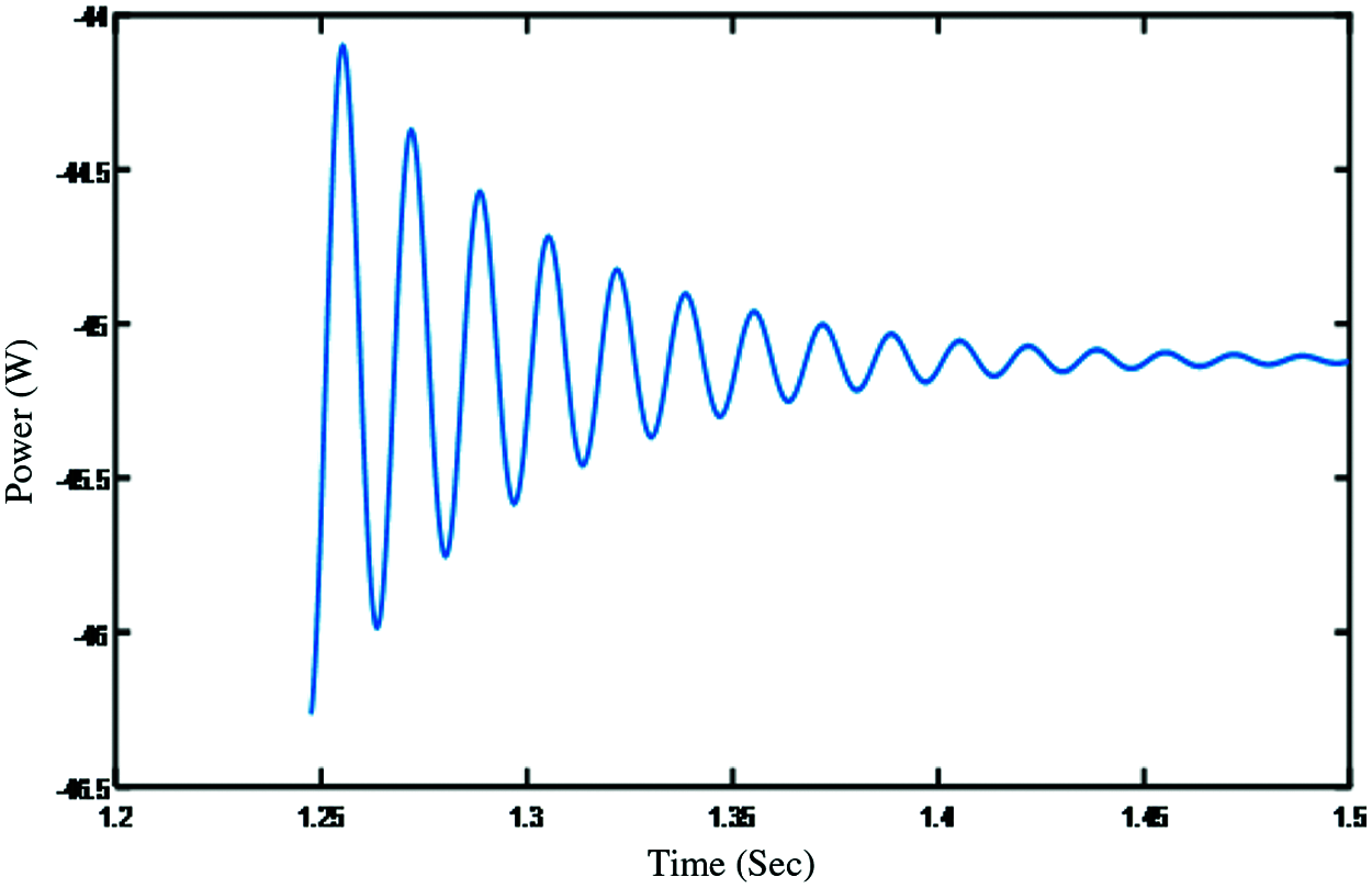
Figure 14: Output power of PID controller
4.3 Proposed FoPID Based GWO Technique
Simulink waveform of input power, irradiance, input dc voltage to PV panel based on FOPID controller is shown in Fig. 15. Fig. 16 gives the output voltage of FOPID controller. The output power of the grid connected inverter based on the FOPID controller is 1598 kW and this is shown in Fig. 17. As the active and reactive power output is shown in Fig. 18.
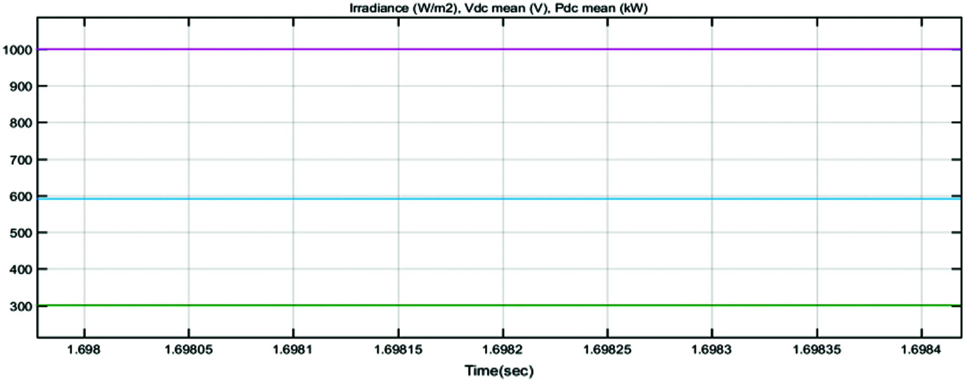
Figure 15: Input power, irradiance, input dc voltage to PV panel based on FOPID controller
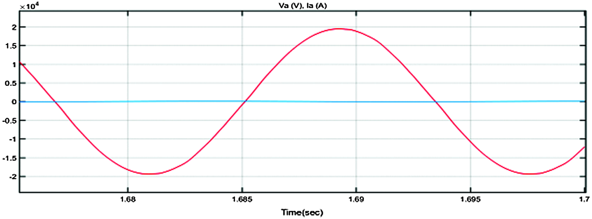
Figure 16: Output voltage with FoPID

Figure 17: AC output power of converter with FOPID controller

Figure 18: Active and reactive power output
4.4 FOPID Based Fuzzy Logic Controller
Tracking of the highest power point and levels of irradiation below 1000W/m2 and 500W/m2. In Fig. 19, the current, voltage and power output of the PV system is given along with the after-effect simulation of the PV system with enhanced MPPT-based fuzzy logic control.

Figure 19: Output of irradiance, voltage, power
.
Fig. 20 shows the input given to fuzzy FOPID controller and the simulink waveform of output voltage, current with Fuzzy FOPID controller is in Fig. 21. Fig. 22 shows Fuzzy based FOPID controller output power of the converter. The output power of the grid connected inverter based on the Fuzzy FOPID controller is 187 kW. The respective solution curve of active and reactive power output from PV system is described in Fig. 23.
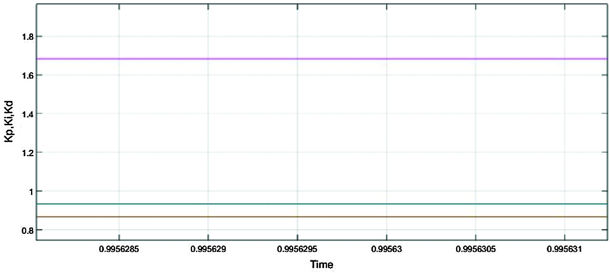
Figure 20: Input to Fuzzy FOPID controller
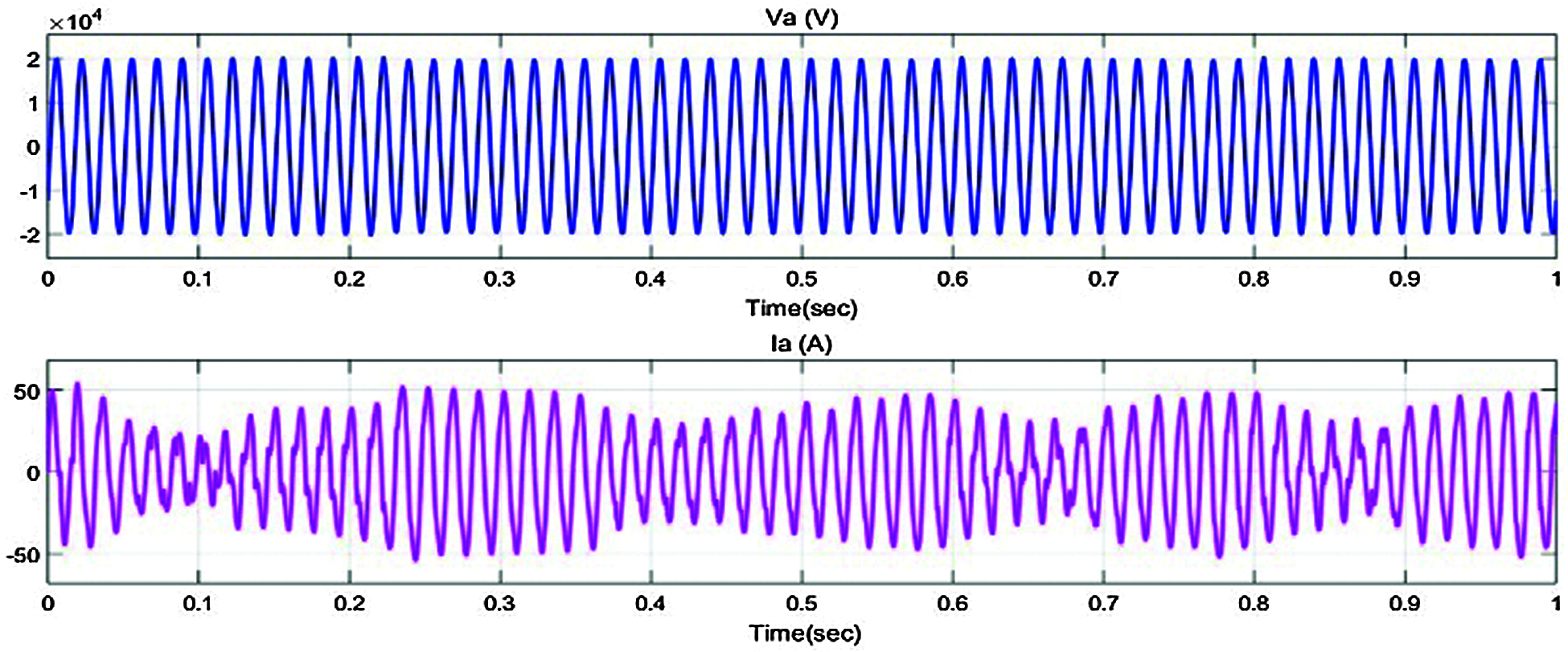
Figure 21: Output voltage, current with Fuzzy FOPID controller
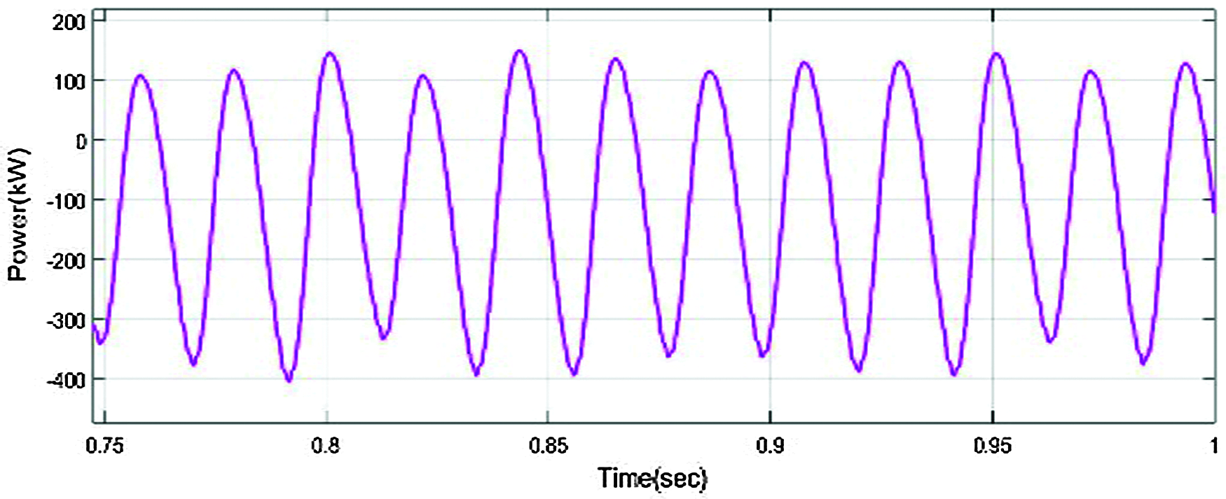
Figure 22: AC output power of converter using fuzzy FOPID controller
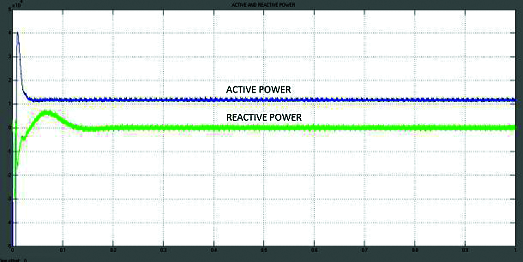
Figure 23: Solution curve of Active and reactive power output from PV system
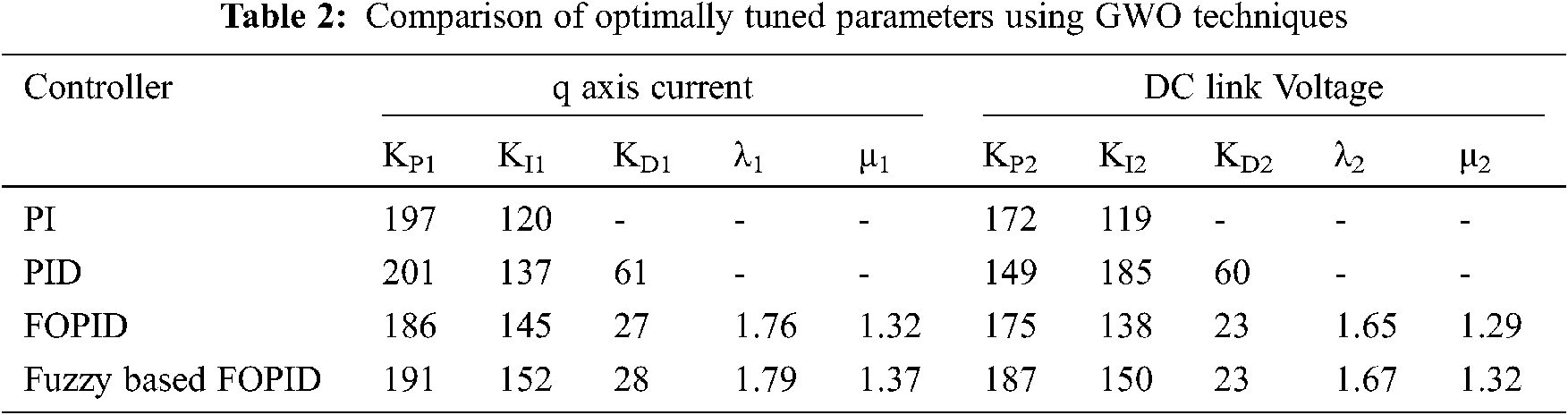
4.5 Comparison of the Proposed Work
The Fuzzy-based FOPID control output is evaluated from the suggested work and contrasted with that of PI, PID control, and FOPID control respectively. The comparison using GWO techniques is illustrated in Tab. 2.
The efficiency comparison graph is shown in Fig. 24. It is inferred that the proposed Fuzzy FOPID outperforms other algorithms in terms of efficiency.

Figure 24: Efficiency comparison of the injected reactive power of the grid connected inverter The efficiency comparison graph is shown in Fig. 24. It is inferred that the proposed Fuzzy FOPID outperforms other algorithms in terms of efficiency
A Fuzzy FoPID energy reshaping control is designed and intended for a grid-connected PV inverter in electric vehicles to optimally extract PV energy under different operating conditions.The performance of current control loop in a three-phase grid-connected PV system has been improved. The performance of current control loop and voltage regulation in a three-phase grid-connected PV system has been dissected. The optimization technique Simulink results show that under different atmospheric conditions, Fuzzy FoPID control can achieve superior control efficiency of 98% with the low control costs as compared to the techniques existing in the literatures. The inverter design in the proposed research can be effectively used in electric vehicles.
The efficiency of current control loops in a three-phase grid-connected PV system has been enhanced by using a fractional order PID controller with other optimization techniques.
Acknowledgement: The authors with a deep sense of gratitude would thank the supervisor for his guidance and constant support rendered during this research.
Funding Statement: The authors received no specific funding for this study.
Conflicts of Interest: The authors declare that they have no conflicts of interest to report regarding the present study.
1. W. Mitkowski and K. Oprzedkiewicz, “Tuning of the half-order robust PID controller dedicated to oriented PV system,” Lecture Notes Electr Eng, vol. 320, pp. 145–157, 2015. [Google Scholar]
2. H. S. Ramadan, “Optimal fractional order PI control applicability for enhanced dynamic behavior of on-grid solar PV systems,” International Journal of Hydrogen Energy, vol. 42, no. 7, pp. 4017–4031, 2017. [Google Scholar]
3. A. Messai, A. Mellit, A. Guessoum and S. Kalogirou, “Maximum power point tracking using a GA optimized fuzzy logic controller and its FPGA implementation,” Solar Energy, vol. 85, no. 1, pp. 265–277, 2011. [Google Scholar]
4. D. Lalili, A. Mellit, N. Lourci, B. Medjahed and C. Boubakir, “State feedback control and variable step size MPPT algorithm of three-level grid-connected photovoltaic inverter,” Solar Energy, vol. 98, pp. 561–571, 2013. [Google Scholar]
5. K. Ishaque, Z. Salam, M. Amjad and S. Mekhilef, “An improved particle swarm optimization (PSO)-based MPPT for PV with reduced steady-state oscillation,” IEEE Transactions on Power Electronics, vol. 27, no. 8, pp. 3627–3638, 2012. [Google Scholar]
6. J. Ahmed and Z. Salam, “A maximum power point tracking (MPPT) for PV system using cuckoo search with partial shading capability,” Applied Energy, vol. 119, no. 12, pp. 118–130, 2014. [Google Scholar]
7. H. Rezk and A. Fathy, “Simulation of global MPPT based on teaching-learning-based optimization technique for partially shaded PV system,” Electrical Engineering, vol. 99, no. 3, pp. 847–859, 2017. [Google Scholar]
8. M. A. Salam, R. Kamel, M. Khalaf and K. Sayed, “Analysis of over current numerical- relays for protection of a stand-alone PV system,” in Proc. SASG, IEEE, Jeddah, Saudi Arabia, pp. 1–6, 2015. [Google Scholar]
9. A. Q. A. Shetwi, M. Z. Sujod and F. Blaabjerg, “Low voltage ride-through capability control for single-stage inverter-based grid-connected photovoltaic power plant,” Solar Energy, vol. 159, pp. 665–681, 2018. [Google Scholar]
10. H. Bounechba, A. Bouzid, H. Snani and A. Lashab, “Real time simulation of MPPT algorithms for PV energy system,” International Journal of Electrical Power and Energy System, vol. 83, pp. 67–78, 2016. [Google Scholar]
11. A. Kchaou, A. Naamane, Y. Koubaa and N. M’sirdi, “Second order sliding mode-based MPPT control for photovoltaic applications,” Solar Energy, vol. 155, pp. 758–769, 2017. [Google Scholar]
12. S. W. Liao, W. Yao, X. N. Han, J. Y. Wen and S. J. Cheng, “Chronological operation simulation framework for regional power system under high penetration of renewable energy using meteorological data,” Applied Energy, vol. 203, pp. 816–828, 2017. [Google Scholar]
13. Y. Wang and B. Ren, “Fault ride-through enhancement for grid-tied PV systems with robust control,” IEEE Transactions on Industrial Electronics, vol. 65, no. 3, pp. 2302–2312, 2018. [Google Scholar]
14. R. L. Tang, Z. Wu and Y. J. Fang, “Configuration of marine photovoltaic system and its MPPT using model predictive control,” Solar Energy, vol. 158, pp. 995–1005, 2017. [Google Scholar]
15. B. Yang, L. Jiang, L. Wang, W. Yao and Q. H. Wu, “Nonlinear maximum power point tracking control and modal analysis of DFIG based wind turbine,” International Journal of Electrical Power and Energy System, vol. 74, pp. 429–436, 2016. [Google Scholar]
16. W. Yao, L. Jiang, J. Y. Wen, Q. H. Wu and S. J. Cheng, “Wide-area damping controller for power system inter-area oscillations: A networked predictive control approach,” IEEE Transactions on Control Systems Technology, vol. 23, no. 1, pp. 27–36, 2015. [Google Scholar]
17. A. Kanchanaharuthai, V. Chankong and K. A. Loparo, “Transient stability and voltage regulation in multimachine power systems vis-à-vis STATCOM and battery energy storage,” IEEE Transactions on Power Systems, vol. 30, no. 5, pp. 2404–2416, 2015. [Google Scholar]
18. R. Kadri, J. P. Gaubert and G. Champenois, “An improved maximum power point tracking for photovoltaic grid-connected inverter based on voltage-oriented control,” IEEE Transactions on Industrial Electronics, vol. 58, no. 1, pp. 66–75, 2011. [Google Scholar]
19. M. Dehghani, M. Taghipour, G. B. Gharehpetian and M. Abedi, “Optimized fuzzy controller for MPPT of grid-connected PV systems in rapidly changing atmospheric coditions,” Journal of Modern Power Systems and Clean Energy, vol. 9, no. 2, pp. 376–383, 2021. [Google Scholar]
20. S. Singh, V. K. Tayal, H. P. Singh and V. K. Yadav “Fractional control design of renewable energy systems,” in Proc. ICR, ITO, Noida, India, pp. 224–231, 2020. [Google Scholar]
21. S. C. Wang, H. Y. Pai, G. J. Chen and Y. H. Liu, “A fast and efficient maximum power tracking combining simplified state estimation with adaptive perturb and observe,” IEEE Access, vol. 30, no. 5, pp. 155319–155328, 2020. [Google Scholar]
 | This work is licensed under a Creative Commons Attribution 4.0 International License, which permits unrestricted use, distribution, and reproduction in any medium, provided the original work is properly cited. |