Intelligent Automation & Soft Computing DOI:10.32604/iasc.2022.021017
Article

Deep Learning-Based Decoding and AP Selection for Radio Stripe Network

Aman Kumar Mishra and Vijayakumar Ponnusamy*

Department of ECE, SRMIST, Chengalpattu, 603203, India
*Corresponding Author: Vijayakumar Ponnusamy. Email: vijayakp@srmist.edu.in
Received: 19 June 2021; Accepted: 04 August 2021

Abstract: Cell-Free massive MIMO (mMIMO) offers promising features such as higher spectral efficiency, higher energy efficiency and superior spatial diversity, which makes it suitable to be adopted in beyond 5G (B5G) networks. However, the original form of Cell-Free massive MIMO requires each AP to be connected to CPU via front haul (front-haul constraints) resulting in huge economic costs and network synchronization issues. Radio Stripe architecture of cell-free mMIMO is one such architecture of cell-free mMIMO which is suitable for practical deployment. In this paper, we propose DNN Based Parallel Decoding in Radio Stripe (DNNBPDRS) to decode the symbols of User Equipments (UEs) in the uplink in a parallel fashion to reduce computational complexity by reducing delay in processing. Moreover, to solve the issue of Access Point (AP) selection in radio stripe networks, we propose a Channel link-based AP selection (CLBAPS) algorithm to choose the best APs in terms of channel link quality. The proposed DNNBPDRS framework not only improves Symbol Error Rate (SER) performance when compared to counterparts but is also proved to be comparatively far lesser computational complex. Moreover, the numerical result indicates the proposed AP selection algorithm CLBAPS performs better than random selection of AP in radio stripe networks.

Keywords: Cell-free massive MIMO; deep learning decoding; beyond 5G; radio stripe; AP selection

1  Introduction

Massive MIMO (mMIMO) is a key wireless physical layer technology in 5G and beyond 5 G (B5G) networks [1], given the features it offers, very high spectral efficiency (SE) by at least ten times [2], improve the radiated energy efficiency [3–6]. However, the adoption of mMIMO (in the current cellular network) faces two major issues. Firstly, as more numbers of antenna is being installed at the base station (mMIMO), inter-cell interference is becoming major bottle neck, this is because inter-cell interference is inherent to cellular paradigm [7]. Secondly, mMIMO suffers from large variations in signal-to-noise ratio between cell-center and cell-edge users [8].

The above-mentioned issues restrict the adoption of mMIMO in beyond 5G (B5G) networks, which is resolved by Cell-Free mMIMO network wherein Central processing unit (CPU) is connected to access point (APs), which jointly serves the given set of User Equipments (UEs) (or all UEs) in the network [9–11]. Authors in [11] discuss the different architecture of cell-free massive MIMO, where they claim centralized implementation of cell-free massive MIMO ‘Level 4’, which performs best in terms of spectral efficiency compared to other architectures. Here, all APs sent their respective received signals in the uplink to CPU over parallel front-haul, which process all the received signals., this requires dedicated front-haul and power supply to each AP, which imposes huge economic costs. Moreover, attaining network synchronization in Cell-Free mMIMO network would be extremely challenging since each AP is connected to CPU over parallel front-haul.

One promising architecture for practical implementation of Cell-free network is using radio stripe [12]. Radio stripes can be easily deployed at public place, stadium, transport (train, bus, etc.) to provide truly ubiquitous connectivity everywhere. Moreover, radio stripe is extremely flexible to deploy, does not require highly trained personnel, needs one connection either to fronthaul or directly to CPU [12].

1.1 Related Works

Given the architecture of radio stripe, where APs are connected sequentially and CPU being connected to last AP (daisy chain architecture) the sequential processing becomes obvious choice. Therefore, authors [13] propose sequential uplink processing for cell-free massive MIMO based on radio stripe. Here, each AP computes the local channel estimate in the uplink, make soft estimate of the transmitted signal and thereby forwards local CSI estimate, soft estimate and error statistic to next AP. Upon receiving the information from the previous AP, the AP improves its own soft estimate. This sequential processing goes on till the last AP, the final estimate is forwarded to CPU for final decoding. Authors [13] claim the proposed processing mechanism achieves comparable performance to ‘Level 4’, while using 90% less signaling in the front-haul. In [8], authors propose Optimal Sequential Linear Processing (OSLP), an uplink sequential processing algorithm which they prove optimal both in the maximum spectral efficiency sense and minimum Mean Square Error (MSE) sense.

However, sequential processing leads to higher processing latency [14]. Therefore, authors in [14] propose two parallel processing schemes in the Radio Stripe network, namely interference-aware MR processing and distributed regularized zero-forcing (D-RZF). Authors [15], propose Q-LMMSE, which implements MRC processing leading to low front-haul loading, simple AP hardware and fast parallel computations.

1.2 Motivation

All works discussed so far in cell-free massive MIMO based on radio stripe [8,13–15] has huge computational needs (for example channel estimation), since next generation network will involve large numbers of APs and UEs. These high computational costs can only be reduced by the application of Deep Learning (DL). DL replaces the complex computations with the trained model, which reduces the complexity considerably.

Authors in [16] propose DeepSIC, which is a data-driven technique for detecting symbols in the Multi-User MIMO (MU-MIMO) scenario. It is based on an iterative SIC algorithm, a MIMO-based detection scheme. Results show it outperforms Iterative SIC in the presence of CSI uncertainty. Since it is an iterative approach, detection is carried out in iteration in a single base station (BS). Our other works on interference cancellation are for Software Defined Radio (SDR) platform [17]. Motivated by the above [16], in our previous work [18], we propose DNN-based distributed sequential uplink processing (DBDSUP) for detecting symbols in the uplink of Cell-Free massive MIMO System Based on Radio Stripe. Here, each AP consists of K (numbers of UEs) parallel Soft Estimate Network (SEN), which computes the conditional distribution of each user at each AP (each AP carries out a single iteration). The conditional distribution of each user consists of the estimation of each symbol in the constellation. The Symbol Error Rate (SER) of the proposed mechanism ‘DBDSUP’ is evaluated. However, the processing here is sequential.

In order to take advantage of DL (to reduce computational complexity) and parallel processing (to reduce latency) there is need to develop a mechanism which is based on DL and does parallel processing.

Moreover, next-generation radio stripe network would involve large numbers of APs (typically in the range of 1000 s in particular give area like train, the bus as shown in Fig. 2), if all APs sequentially decodes transmitted symbol of given user, it would impose huge complexity on the system. Therefore, it becomes extremely important to develop a mechanism for users to select APs in Cell-free massive MIMO based on radio stripe.

Authors in [19] propose an effective channel gain-based algorithm in massive cell-free MIMO to assign users to each AP sequentially. Here author considers two metrics, first measure the channel quality of each user to all APs, and another one is to calculate the effective channel gain between every user and AP in the system, which reduces interferences and leads to a higher sum rate. Other works on AP selection focus on Machine learning (ML) [20].

This paper aims to propose a deep learning-based parallel decoding mechanism and AP selection algorithm for cell-free massive MIMO based on radio stripe.

1.3 Contributions

The contribution is stated in the points below.

•   We propose DNN based Parallel Decoding in Radio Stripe (DNNBPDRS). This has two benefits, firstly, DNN processing (reduces the computational complexity) and secondly, parallel processing reduces the latency, making it very attractive for beyond 5G (B5G) technology (radio stripe is slated to be 6th generation wireless technology).

•   To solve the issue of AP selection in the radio stripe network. We propose a Channel link-based AP selection (CLBAPS) algorithm to choose the best APs (in terms of channel link quality).

The rest of the paper is organized as follows. In Section 2, we discuss the network model of radio stripe . Section 3, elaborate about different aspect of proposed DNN based Parallel Decoding in Radio Stripe (DNNBPDRS). In Section 4, a detailed description of the proposed AP selection algorithm, Channel link-based AP selection (CLBAPS), is detailed. Simulation setup, training of neural network and numerical results are discussed in Section 5. Finally, the article is concluded in Section 6.

2  Radio Stripe Network Model of Cell-Free Massive MIMO

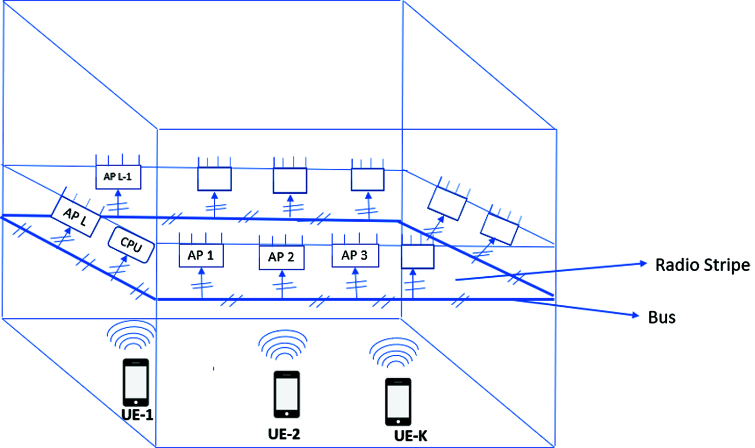
Figure 1: Radio stripe network model

Fig. 1 shows ‘radio stripe’ network model, which consists of L APs (all APs are connected sequentially as shown in Fig. 1), with CPU being connected to the last AP (Lth AP). The fronthaul connections are given by AP1->AP>………….->APL->CPU. K single antenna User Equipments (UEs) are randomly distributed. Each AP consists of N numbers of antenna. As shown in Fig. 1, radio stripe is easy to deploy since it is light in weight and extremely flexible to deploy, which makes it possible to be deployed in any place like office, public place, stadium, etc., as also depicted in Fig. 2.

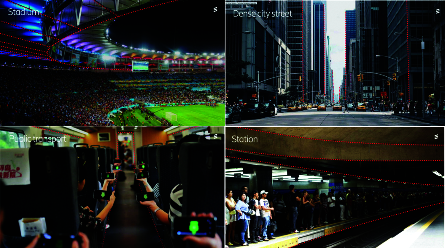
Figure 2: Different scenarios of radio stripe deployment

The channel gain between kth UE and nth antenna of lth AP is given by [21],

glnk=Llnk−bFlnk12hlnk (1)

Llnk=||dlnk|| is the Euclidean distance between kth UE and nth antenna of lth AP, b is the path-loss exponent. Flnk=10σlnkzlnk10 is log-normal shadowing correlation factor, with a standard deviation of σlnk and zlnk=δalnk+1−δblnk , where alnk and blnk ~ N(0, 1) are i.i.d random variables (rvs) which represents shadow fading effect at UE k and nth antenna in lth AP and δ is the transmitter-receiver shadow fading correlation coefficient. hlnk is the small-scale channel fading between kth UE and nth antenna of lth AP and follows independent but not identically distributed (i.n.d) Nakagami-Mlnk distributions with shape and spreading parameters Mlnk and Ωlnk . Since hlnk has Nakagami distribution hence |hlnk|2 has gamma distribution, i.e. |hlnk|2 ~G ( αlnk,βlnk ), where αlnk=Mlnk is shape parameter and βlnk = ΩlnkMlnk is scale parameters respectively.

It is assumed that Llnk and Flnk are known. Therefore, we have |glnk|2 ~ G( αlnk,β′lnk ) where β′lnk=βlnkLlnk−2bFlnk=βlnkLlnk2bFlnk=ΩlnkLlnk2bMlnkFlnk .

The signal received at lth AP is given by,

yl=glnkS+Nl (2)

where S is transmitted symbol vector and consists of transmitted symbol from K UEs which is S = [s1, s2, …,sK]. N ∈ RN × 1 is the noise vector at the lth AP whose entries have distribution with zero mean and variance of σ2 , with σ2 being noise power.

If number of antennas in each AP is 1 (N =1), Eq. (1) can be modified as

glk=Llk−bFlk12hlk (3)

As suggested in literatures [8,13–15], sequential processing is done in radio stripe network. The effective channel estimate of kth UE channel at the Lth AP [8] is given below

g^k=[g^1k,g^2k,g^3k,……..g^Lk] (4)

3  Deep Neural Network-Based Parallel Decoding in Radio Stripe

In this section, we discuss about, Iterative SIC which is the background for our works, the motivation behind applying deep learning in radio stripe, proposed parallel processing radio stripe network model, then we discuss about Soft Estimate Network (SEN), which forms the core of the proposed parallel decoding framework. Lastly, we discuss about the proposed algorithm.

3.1 Iterative SIC

In this subsection, we briefly discuss about iterative Soft Iterative Cancellation (SIC) [22]. Iterative Soft Interference Cancellation (SIC) is a multi-user detection technique that combines parallel (multi-stage) interference cancellations with soft decoding. In a general sense, iterative SIC is an iteration-based detection scheme wherein each iteration, two operations are carried out in parallel for each user, namely Interference cancellation and soft decoding. Considering Kth user and cth iteration, during the interference cancellation stage, the expected values and variances of {su}u ≠ k (interfering symbols) are computed based on { P^u(c−1) }u ≠ k. Pk(c) is the estimated conditional distribution of kth user symbol sk. Entries of Pk(c) are the estimate of the distribution of sk for each possible symbol in the constellation. { P^u(c−1) }u ≠ k is the estimated conditional distribution of interfering symbols obtained in the previous iteration. The expected value of interfering user in cth iteration is computed as

eu(c−1)=∑rw∈S⁡rw(P^u(c−1))w (5)

where {rw}Ww = 1 are the indexed elements of the constellation set CS. The variance of interfering symbols is given by,

Vu(c−1)=∑rw∈CS⁡(rw−eu(c−1))2 (P^u(c−1))w (6)

The contribution of the interfering symbols from the received signal y is canceled by replacing it with mean {eu(c−1)} and subtracting the resultant term. Considering hu the uth column of H the elements of H with respect to user u. where H is channel matrix of all K user where each column represents one user channel vector. Interference canceled output of the channel is given by,

Gk(c)=y−∑u≠k⁡hueu(c−1) (7)

=hksk+∑u≠k⁡hu(su−eu(c−1))+N (8)

The second step carried out in parallel for each user is soft decoding. The bijective transformation of y is Gk(c) , such that each possible value of y there is one unique value in Gk(c). Therefore, Psk|y(rw|y)=Psk|Gk(c)(rw|Gk(c)) for each rw ∈ CS. Therefore, the conditional distribution of sk given y is approximated from the conditional distribution of Gk(c) given sk using Bayes theorem. Each symbol is equiprobable. Conditional distribution is computed as,

(P^k(c))w=PGk(c)|sk(Gk(c)|rw)∑r′w∈S⁡PGk(c)|sk(Gk(c)|r′w) (9)

Symbols are decoded after the final iteration such that symbol which maximizes estimated conditional distribution is decoded as the transmitted symbol for each user.

s^k=arg⁡max(P^k(C))w (10)

where w ∈ {1, 2, …….., W}

The algorithm in steps is given in our previous works [18].

3.2 Motivation Behind Applying Deep Learning in Radio Stripe

Iterative SIC is leveraged to perform data-driven detection “DeepSIC” in Multi-User MIMO (MU-MIMO) [16], motivated by this work, in our last work, we proposed DNN-based distributed sequential uplink processing (DBDSUP) in cell-Free massive MIMO based on radio stripe by exploiting data-driven iterative SIC. However, it considers sequential processing leading to higher latency, which can be reduced given the processing is carried out in a parallel fashion. Thus, we propose DNN based Parallel Decoding in Radio Stripe (DNNBPDRS), which carries out parallel processing in radio stripe networks.

3.3 Proposed Parallel Processing Network Model

Fig. 3 shows a simplified proposed parallel processing network model.

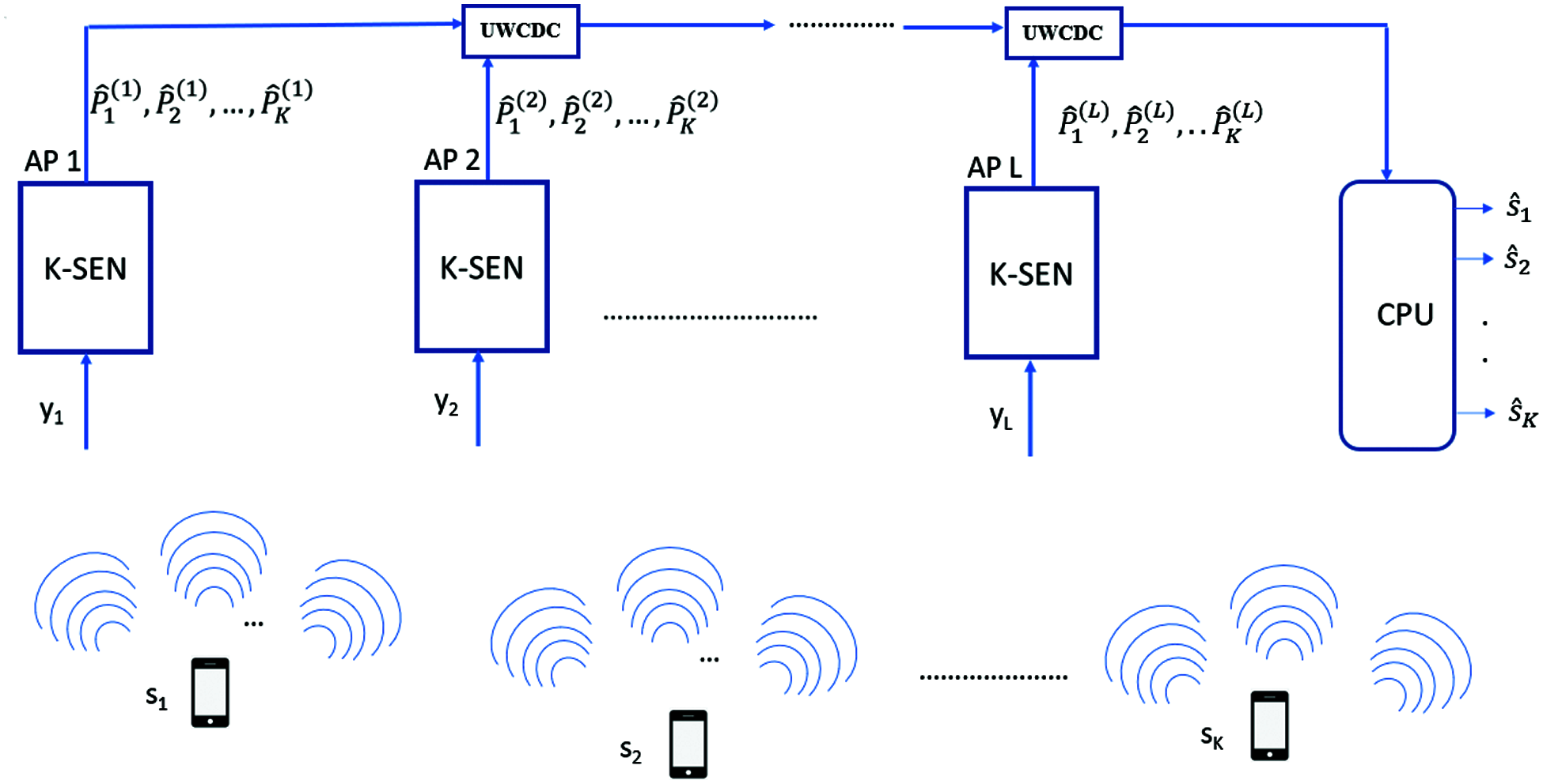
Figure 3: Simplified proposed parallel decoding mechanism

As shown in Fig. 3, each AP consists of K-parallel Soft Estimate Network (SEN) (which is discussed in detail in Section 3.4). As opposed to sequential processing, here each AP process the received signal simultaneously. The signal received at AP1, AP2, ……….., APL is given by y1, y2, …….., yL.

3.4 Soft Estimate Network

As shown in Fig. 4, Soft Estimate Network (SEN) is a classification-based Neural Network. As explained above, iterative SIC carries out two operations in parallel for each user, namely, interference cancellation and soft decoding. In particular, for cth iteration and kth user soft decoding estimate P^K(c) is a classification task since entries of P^K(c) is an estimation of the distribution of kth user symbols for each symbol in the constellation with the dimension of P^K(c) being RB.

SEN replaces these complex computations for each iteration. Moreover, interference cancellation and soft decoding are dependent on the underlying channel model. However, SEN does not require any knowledge of the channel model since it is based on dedicated neural network which is trained for different channel scenarios.

Moreover, the inputs to SEN are yl and Ik(c−1) . Here yl and Ik(c−1) are the received signal at the lth AP and interference coefficient of the kth user during cth iteration, respectively.

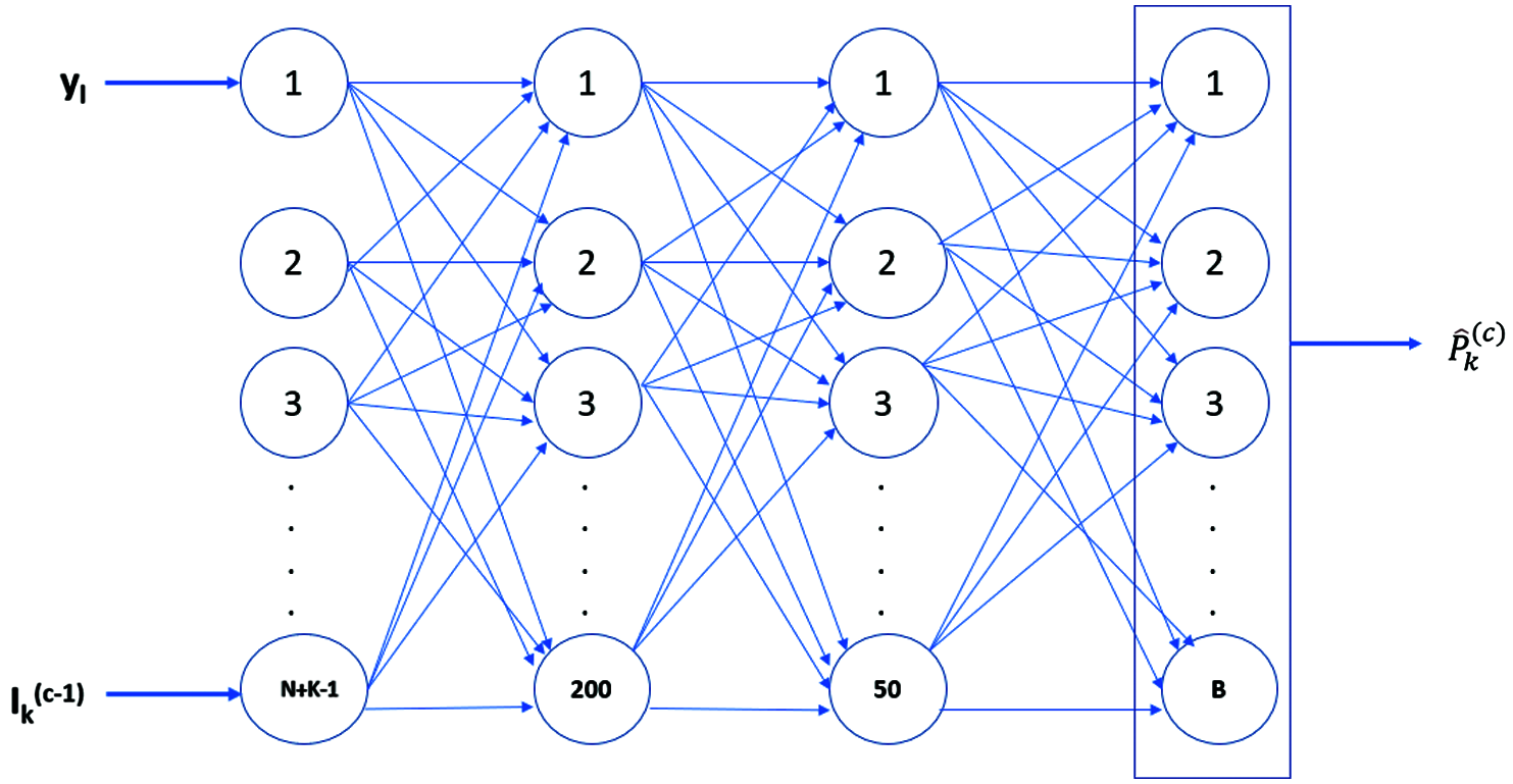
Figure 4: Soft estimate network (SEN)

The last layer of SEN is the Softmax layer; it consists of neurons equal to the numbers of symbols in the constellation. For example, if Binary Phase shift Keying (BPSK) is employed, then the Softmax layer consists of 2 (B) neurons.

3.5 Deep Neural Network-Based Parallel Decoding in Radio Stripe (DNNBPDRS)

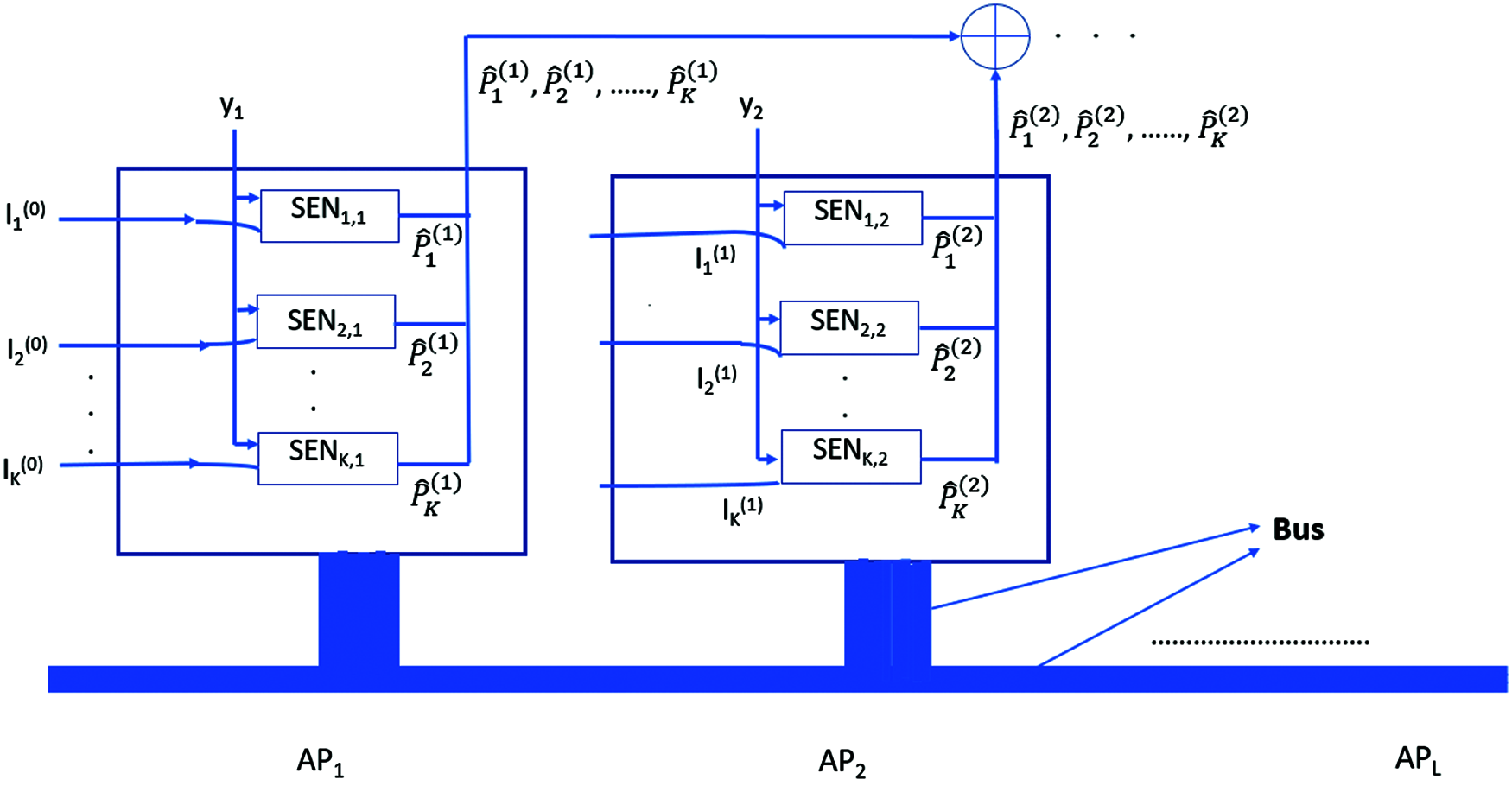
Figure 5: Processing in proposed radio stripe architecture

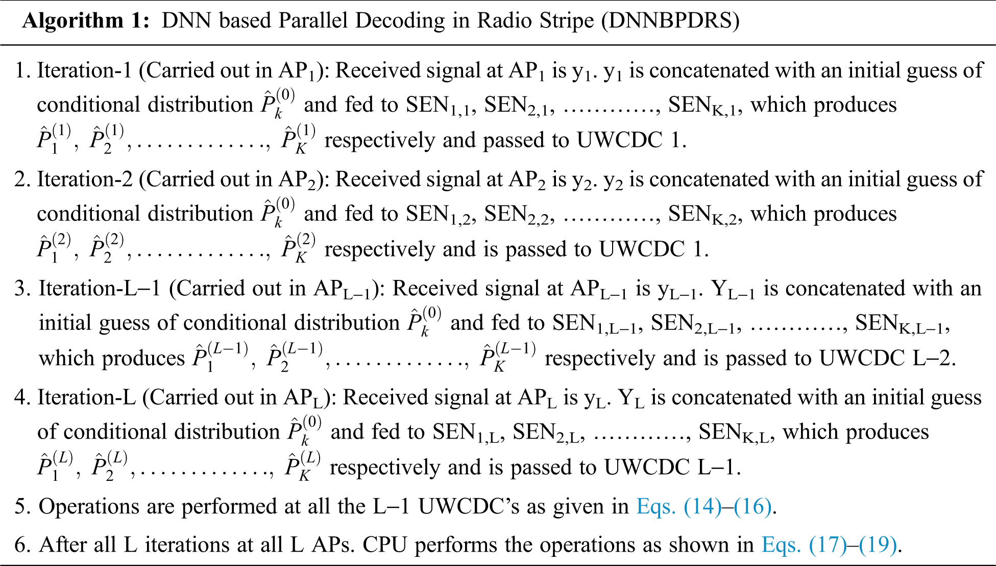
In this subsection, we discuss about the proposed parallel decoding scheme, DNN based Parallel Decoding in Radio Stripe (DNNBPDRS). Fig. 5 shows the K parallel SENs in each AP. As shown in Fig. 5, AP1 receives y1, which forms one of two inputs to SEN1,1, SEN2,1, ……….., SENK,1 (first subscript denotes the kth user and the second subscript denotes the lth AP) while the second input to SENs are interference coefficients I1(0) , I2(0) , …………, IK(0) and takes the value of 1B [16], which are given by

I1(0)=[P^2(0),P^3(0),.........,P^K(0)] (11)

I2(0)=[P^1(0),P^3(0),.........,P^K(0)] (12)

Considering SEN1,1, the SEN belonging to UE 1 at AP1, it receives y1 and I1(0) to produce P^1(1) , the conditional distribution of UE 1. Similarly, SEN2,1 and SEN3,1, produces P^2(0)andP^3(0) respectively as shown in Fig. 5. Likewise, SEN1,2 in AP2 accepts inputs y2 and I1(1) to produce P^1(2) , where I1(1) is given by

I1(1)=[P^2(1),P^3(1),..........P^K(1)] (13)

In a similar way, all SENs in all L APs compute respective conditional distribution. To sum the conditional distribution of L APs, L−1 numbers of User-Wise Conditional Distribution Combiner (UWCDC) is required.

Finally, the UWCDC performs the following operations,

S^1t=P^1(1)+P^1(2)+……….+P^1(L) (14)

S^2t=P^2(1)+P^2(2)+……….+P^2(L) (15)

and,

S^kt=P^k(1)+P^k(2)+……….+P^k(L) (16)

where, S^1t , S^2t and S^kt are the total added conditional distribution of 1st, 2nd and kth user and has the dimension of 1 × B (B is the size of constellation). For instance, if BPSK is considered then B = 2.

For each user the CPU performs the operation given below

S^1=maxcs∈{+1,−1}⁡(S^1t) (17)

S^2=maxcs∈{+1,−1}⁡(S^2t) (18)

and,

S^k=maxcs∈{+1,−1}⁡(S^kt) (19)

Above max operations, choose the symbol from the constellation which has the maximum value. For example, if BPSK constellation is considered and S^1t=[0.15,0.85] , then S^1=0.85 and the decoded symbol is +1.

The total numbers of SENs present in radio stripe is given by NSEN.

NSEN=KL (20)

The proposed DNN based Parallel Decoding in Radio Stripe (DNNBPDRS) is given in steps below.

3.6 Complexity Analysis

This subsection discusses and compares the complexity of proposed DNNBPDRS, DNNBDSD [18] and iterative SIC.

3.6.1 Complexity Analysis of DNNBPDRS

Considering the input layer, SEN has four layers therefore, it needs three matrices to represent weight between these layers. Let the numbers of nodes in 1st, 2nd, 3rd, 4th layers be p, q, r, and s, respectively. The weight matrices are denoted as Wqp, Wrq, Wsr. For example, Wqp contains weights going from layer p to layer q. Considering there are t examples of data that has to be fed to SEN. Forward propagation from the 1st layer to 2nd layer, we have

Xqt=Wqp∗Ipt (21)

where Xqt is the computed calculation at the second layer, Ipt is the input fed to the first layer of SEN having p nodes. The time complexity is given by

O(q∗p∗t) (22)

where O denotes the numbers of the operation carried out at each fully connected layer. After the forward pass, the activation function is applied at the 2nd layer, and since it is an element-wise operation hence time complexity is

O(q∗t) (23)

So, the total time complexity involved in going from the 1st layer of SEN to 2nd layer is

O(q∗p∗t+q∗t) (24)

O(q∗p∗t) (25)

Similarly, time complexity in going from layer 2 to layer

O(r∗q∗t) (26)

Time complexity involved in going from layer 3 to layer 4

O(s∗r∗t) (27)

Therefore, the total time complexity for feed-forward propagation is

O(q∗p∗t+r∗q∗t+s∗r∗t) (28)

O(t∗(pq+qr+rs)) (29)

During the backpropagation, the time complexity is the same as shown in Eq. (29). Hence total time complexity involved in training is as shown in Eq. (29). The proposed DNNBPDRS algorithm consists of NSEN SENs, however, the processing is carried out in parallel fashion. Moreover, SEN is trained for several iterations (epoch) n. So total time complexity for training SENs is

O(n∗t∗(pq+qr+rs)) (30)

However, during the testing and deployment of DNNBPDRS, each input to SEN is passed only once with final detected symbols at the CPU. Therefore, the computation complexity of deployed DNNBPDRS is given by

O(pq+qr+rs) (31)

3.6.2 Complexity Analysis of DNNBDSD

Our previous work DNN-based distributed sequential uplink processing (DBDSUP) [18], also employs SENs, with the only difference being sequential processing.

Therefore, the computational complexity of DNNBDSD can be compared with the computational complexity of DNNBPDRS and remains the same till Eq. (31). However, DNNBDSD carries out sequential processing and the radio stripe consists of NSEN SENs. Therefore, the computation complexity of deployed DNNBDSD is given by

O(NSEN∗(pq+qr+rs)) (32)

3.6.3 Complexity Analysis of Iterative SIC

In this subsection, we discuss the O complexity of Iterative SIC in order to compare the same with DNNBPDRS and DNNBDSD. Iterative SIC mainly consists of 4 stages, expected value computation, variance computation, interference cancellation and soft decoding. The complexity involved in each step is given below.

For expected value, from Eq.(5), the complexity involved to compute the expected value of interfering users for one particular user is given as

O(2(K−1)+B(K−1)) (33)

For K UEs,

O(K(2(K−1)+B(K−1))) (34)

O(2K2−2K+BK2−BK) (35)

Computation of variance involves similar steps hence the complexity involved in computing variance is also,

O(2K2−2K+BK2−BK) (36)

Thirdly, for interference cancellation from Eq. (8), the complexity involved in computing interference cancelled output for one particular user is given by

O((K−2)+(K−1)) (37)

For K UEs,

O(2K2−3K) (38)

Lastly, Computational complexity involved in computing soft decoding for one user is

O(B)

For K UEs

O(KB) (39)

Time complexity involved in four stages at one AP is hence given by

O(6K2−7K+2BK2−BK) (40)

Since these computations are carried out for C iterations (as given in iterative SIC algorithm) at each AP and carried out at L AP, hence complexity is given as

O(LC(6K2−7K+2BK2−BK)) (41)

Moreover, iterative SIC requires full CSI, let the time complexity involved in acquiring full CSI for one user be given as CA, therefore time complexity for acquiring CSI for K users at L AP is given by,

O(LK(CA)) (42)

Hence, total time complexity involved in iterative SIC is

O(LC(6K2−7K+2BK2−BK)+LK(CA)) (43)

Comparing Eqs. (31), (32) and (43), since Eq. (43) is polynomial, therefore it is very evident that complexity of iterative SIC detector is higher than proposed DNNBPDRS and DNNBDSD. Moreover, as seen from Eqs. (31) and (32), DNNBDSD has NSEN times more time complexity then DNNBPDRS.

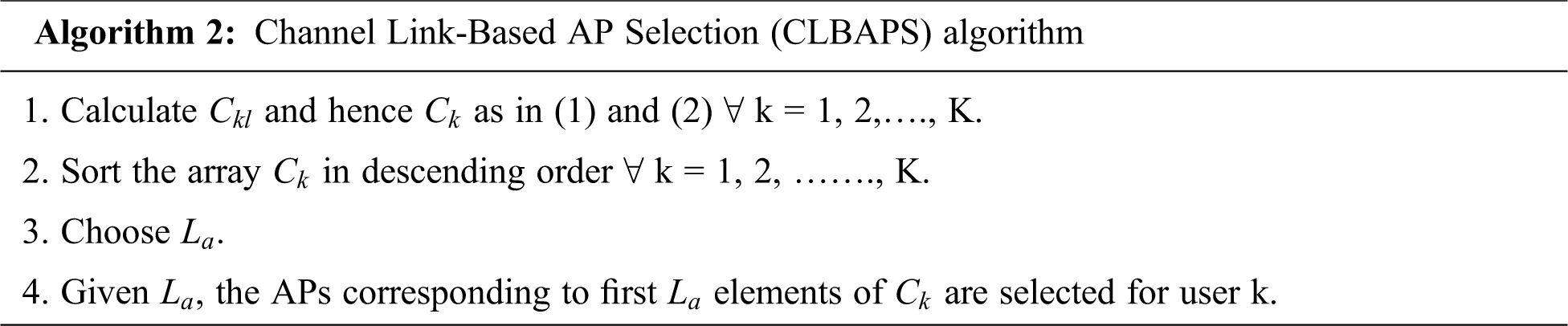
4  Channel Link-Based AP Selection Algorithm

The SINR in the uplink of user k at lth AP given by,

γku=∑n=1N⁡Pk|g^k|2∑n=1N⁡[∑u=1,u≠kK⁡Pu|g^u|2]+σnu2 (44)

where, Pk is transmitted power of user k in uplink and σnu2 is effective noise power. Hence, Up Link (UL) spectral efficiency is given by,

SEu=τuτc∑k=1K⁡log2(1+γku) (45)

where τu is UL transmission phase and τc is coherence interval. Channel link metric-Channel link is basically the numerator component of SINR, which determines the channel gain between UE and AP.

Channel Link between kth user and lth AP is given below,

Ckl=|g′lnk|2 (46)

For each UE k an array of channel link consisting of L elements is, in particular

Ck=[CLk1,CLk2,………………,CLkL] (47)

Let the numbers of APs to which UE k is connected in the uplink be given by La . UE k accesses these La AP sequentially.

We propose channel link-based algorithm to choose the most suitable APs. In the step 1 and 2 channel links for each user is calculated and sorted in descending order. Based on the chosen La in step 3, the APs corresponding to first La are chosen for user k in step 4. To ensure fair usage for all users, all four steps are carried in parallel fashion for each user.

The proposed AP selection algorithm is summarized in algorithm 3 below.

5  Numerical Results

In this section, we discuss on simulation parameters, the performance of the proposed decoding scheme DNNBPDRS, complexity analysis of DNNBPDRS and finally, we discuss the performance of the proposed channel selection algorithm CLBAPS.

5.1 Simulation Setup

For large-scale fading, we assume that all users are randomly distributed over a stadium of circular shape with a radius 10 m which corresponds to the total coverage area of 314 m2. Radio stripe is installed across the circumference of the stadium at a height of 5 m from the ground.

5.2 Training of SEN

The symbols are randomly derived from BPSK Constellation Set (CS) ∈ {0, 1}, which undergoes operation as given by Eq. (2). For each particular value of yl at all the APs, SENs across all APs are trained in a parallel manner. The SENs across all APs are trained on 20 K samples. At lth AP, the received signal is y1, based on the initial estimate {P^k(0)}k=1K all K SENs in each AP are trained in a parallel fashion for all 20 K samples.

For a given transmitted symbol vector S, all SENs across all APs are trained in a parallel fashion. Since the proposed DNNBPDRS is trained via supervised learning, the label (actual conditional distribution) corresponding to the transmitted symbol vector is available to compute loss.

Since, SEN1,1 has a softmax layer as the output layer, the output at each neuron of the softmax layer is given as

exp(xi)∑j=1B⁡(xj) (48)

where (xi) and (xj) are elements of P^1(1) .

Let ∅ represents weight and biases of SEN1,1. Since, P1(1) consists of B elements, P1(1)=[O1,O2,……….,OB] . The loss function at the output of SEN1,1 is defined as

L(∅)=−∑i=1B⁡(P1(1))ilog⁡(P^1(1))i (49)

where P1(1) and P^1(1) are the actual conditional distribution and estimated conditional distribution respectively. The parameter ∅ are updated using Adam optimizer and is defined as

∅f+1=∅f−ηmfvf+∈ (50)

η is Learning rate. ∈ is a smoothing term which prevents divisions by 0. mf and vf are the estimate of the mean (first moment) and uncentered variance (second moment) of the gradients and is given as,

mf=β1mf−1+(1−β1)∇L(∅f) (51)

v=β2vf−1+(1−β2)∇[L(∅f)]2 (52)

β1 and β2 are the decay rates of the moving average. Similarly, all SENs across all APs are trained in a sequential manner.

5.3 Analysis of DNNBPDRS

In this subsection, we analyze the performance of the proposed DNNBPDRS algorithm and compare its performance with Cell-Free massive MIMO ‘Level 4’ implementing iterative SIC [11] under CSI uncertainty and our proposed sequential processing in radio stripe [18]. It is quite evident from Fig. 6, the best performance is achieved by the proposed DNNBPDRS algorithm.

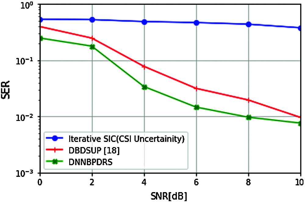
Figure 6: Symbol Error Rate (SER) performance of proposed framework

Considering the numerical difference in Symbol Error Rate (SER) performance of the three frameworks are compared, the percentage difference of DNNBPDRS-iterative SIC and DNNBPDRS-DBDSUP are 99.05% and 32.72%, respectively for 2dB Signal-to-Noise Ratio (SNR).

For 8dB SNR, the percentage difference of DNNBPDRS-iterative SIC and DNNBPDRS-DBDSUP are 191.35% and 132.53%, respectively. For all SNRs the difference between DNNBPDRS-iterative SIC is much higher than DNNBPDRS-DBDSUP.

The better performance of DNNBPDRS then DBDSUP is attributed to the fact that in DNNBPDRS, each AP is trained for five iterations, while in DBDSUP each AP is trained for a single iteration. Moreover, in DBDSUP there are chances that errors in conditional distribution estimation may propagate from one AP to next AP, which is eliminated completely in DNNBPDRS.

Since, we consider radio stripe to be deployed across the walls of room/stadium as indicated in Fig. 2, it becomes important to determine the decoding performance of the proposed DNNBPDRS framework for different numbers of AP L, given the numbers of UEs present in the radio stripe network. Therefore, we analyze the performance of DNNBPDRS with different numbers of APs L for a given number of UEs K in the network.

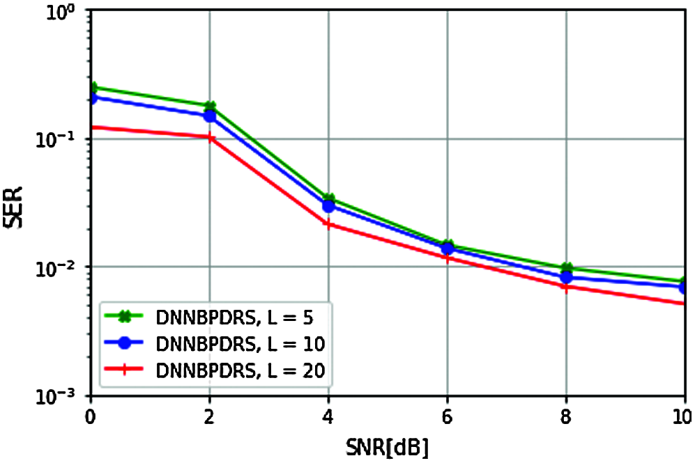
Figure 7: SER performance of DNNBPDRS for different numbers of APs L

Simulation is carried out for three different numbers of APs L using the simulation parameters given in Tab. 1. In particular, simulation is carried out for L = 5, L =10 and L = 20. Tab. 2 shows the percentage of difference in obtained SER.

As the number of AP L increases, the performance of DNNBPDRS improves. Tab. 2 shows the percentage difference in SER achieved for different combinations. It can be clearly noted for the second combination L = 5, L = 20 (the difference being 4 times), the percentage difference is highest.

Moreover, it can be clearly observed from Fig. 7, that the performance of the proposed DNNBPDRS improves as L > K inequality increases.

5.4 Analysis of Channel Link-Based AP Selection

Figure 8: CDF of spectral efficiency with L = 10, La = 4

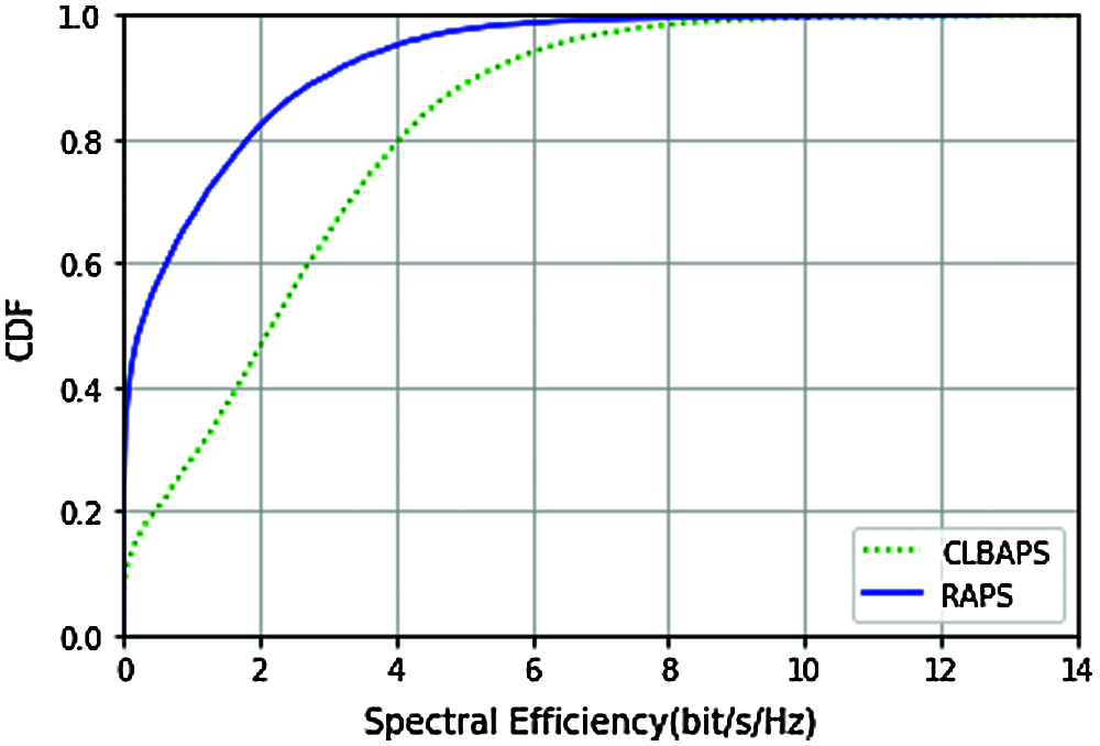
Figure 9: CDF of spectral efficiency with L = 20, La = 4

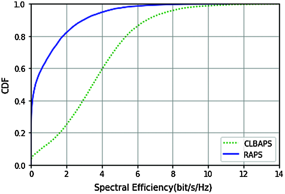
Figure 10: CDF of spectral efficiency with L = 50, La = 4

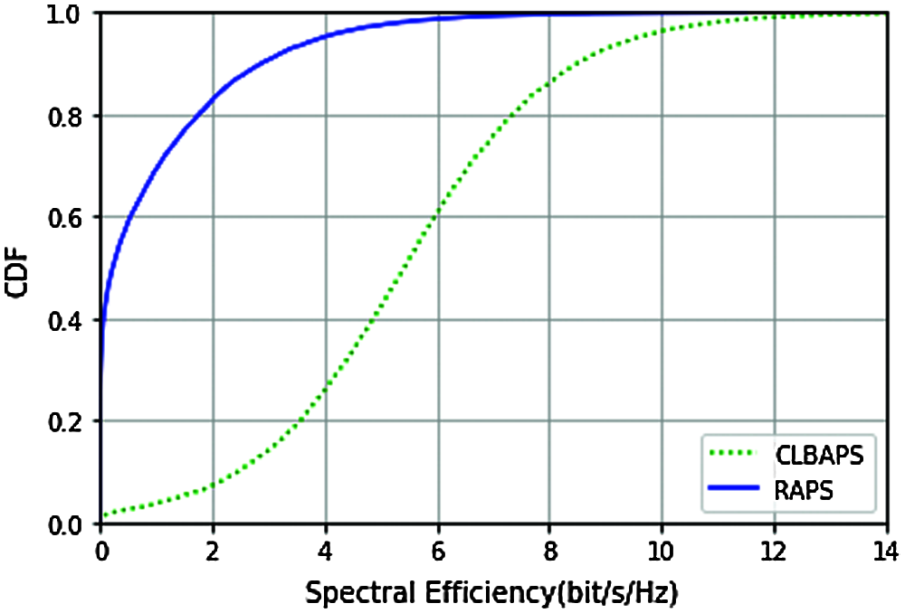
Figure 11: CDF of spectral efficiency with L = 200, La = 4

The above four figures (Figs. 8–11) compare the CDF of proposed Channel-link based AP selection (CLBAPS) with CDF of Random AP selection (RAPS) (here AP are selected randomly). Analysis is carried out for different numbers of AP L in the radio stripe network, keeping La constant. It can be clearly observed the gap between the proposed scheme and random selection increases as the numbers of AP in the network increases. In particular, from Fig. 8, the proposed CLBAPS algorithm gains 0.960 bit/s/Hz as compared to the RAPS with 50% probability. While with the proposed algorithm the SE of the UEs with 50% probability have 5.261 bit/s/Hz gain over random selection, when L = 200. The reason for these results is quite obvious, as the numbers of APs in the network increases there are more chances of UE being close to AP with excellent channel link. However, there is insignificant impact of increase in numbers of AP L for random AP selection as it gains 0.0383 bit/sec/Hz when increasing the APs in the network from 10 to 200.

6  Conclusion

Cell-Free massive MIMO is slated to be beyond 5G (B5G) technology; however, its practical adoption issues mar its implementation. Radio stripe, an architecture of cell-free massive MIMO is suitable for practical implementation and is envisioned to be 6G technology by industry experts. In this paper, we propose, deep learning-based parallel decoding scheme in cell-free massive MIMO based on radio stripe namely DNN based Parallel Decoding in Radio Stripe (DNNBPDRS), which gives two benefits. Firstly, DNN processing reduces the computational complexity and secondly, parallel processing reduces the latency, making it very attractive for 6th generation wireless technology. Moreover, to solve the issue of AP selection in radio stripe network. We propose Channel link-based AP selection (CLBAPS). In the future, more research can be carried out to optimize the parallel processing in radio stripe, which would further reduce the computational complexity and allow UEs to choose the best APs for uplink processing by considering different simulation setups and different parameters such as distance and mobility.

Funding Statement: The authors received no specific funding for this study.

Conflicts of Interest: The authors declare that they have no conflicts of interest to report regarding the study.

This work is licensed under a Creative Commons Attribution 4.0 International License, which permits unrestricted use, distribution, and reproduction in any medium, provided the original work is properly cited.