DOI:10.32604/iasc.2022.021296
| Intelligent Automation & Soft Computing DOI:10.32604/iasc.2022.021296 | |
| Article |
Restoration of Adversarial Examples Using Image Arithmetic Operations
Department of Information Technology, University of Central Punjab, Lahore, 54000, Pakistan
*Corresponding Author: Kazim Ali. Email: kazimravian2003@gmail.com
Received: 28 June 2021; Accepted: 29 July 2021
Abstract: The current development of artificial intelligence is largely based on deep Neural Networks (DNNs). Especially in the computer vision field, DNNs now occur in everything from autonomous vehicles to safety control systems. Convolutional Neural Network (CNN) is based on DNNs mostly used in different computer vision applications, especially for image classification and object detection. The CNN model takes the photos as input and, after training, assigns it a suitable class after setting traceable parameters like weights and biases. CNN is derived from Human Brain's Part Visual Cortex and sometimes performs even better than Haman visual system. However, recent research shows that CNN Models are much vulnerable against adversarial examples. Adversarial examples are input image huts that are deliberately modified, which are imperceptible to humans, but a CNN model strongly misrepresents them. This means that adversarial attacks or examples are a serious threat to deep learning models, especially for CNNs in the computer vision field. The methods which are used to create adversarial examples are called adversarial attacks. We have proposed an easy method that restores adversarial examples, which are created due to different adversarial attacks and misclassified by a CNN model. Our reconstructed adversarial examples are correctly classified by a model again with high probability and restore the prediction of a CNN model. We will also prove that our method is based on image arithmetic operations, simple, single-step, and has low computational complexity. Our method is to reconstruct all types of adversarial examples for correct classification. Therefore, we can say that our proposed method is universal or transferable. The datasets used for experimental evidence are MNIST, FASHION-MNIST, CIFAR10, and CALTECH-101. In the end, we have presented a comparative analysis with other state-of-the methods and proved that our results are better.
Keywords: Computer vision; deep learning; convolutional neural network; adversarial attacks; adversarial examples; and adversarial defense methods
After Khrushchevsky and many others, deep learning became the focus of attention [1]. In 2012 the most challenging large-scale visual recognition task demonstrated the impressive performance based on a CNN [2,3]. Since 2012, Computer vision experts have done a great deal in deep learning research, providing solutions to medical applications problems [4] and mobile applications [5].
The current development of Artificial Intelligence in Tabla-Rasa Learning of Alphago-Zero [6] is due to the Res-Net network [7] initially created for image classification. The growing growth of deep learning models [7–9], availability of free deep learning libraries and APIs, and efficient hardware can easily train difficult models [10–12]. Due to these improvements, deep learning models nowadays are used in automated-driving cars [13], security-based Apps [14], searching-malware [15,16], drone-technology and robot-technology [17,18], language recognition, facial recognition, face-book identity security for smartphones [19,20]. From this, it is proved that deep learning in computer vision applications has played an important role in our daily lives.
The CNNs and DNNs models are much weaker against adversarial examples or attacks. Therefore it is a significant threat against the applications based on CNN's, e.g., autonomous-car, CNNs-based face recognition, DNNs-based malware-detection system [21–23]. After Szegedy et al. [24] ‘s work on adversarial examples, so many adversarial attacks are developed to create adversarial examples to fool different deep learning models, especially in the computer vision field [25–31]. There are two main types of adversarial attacks White-box attacks, i.e., where knowledge of the model's structure and parameters are available, and Black-box attacks, i.e., where an adversary (attacker) does not know the CNN model. If an adversarial example is fooled by other CNNs models also, then this property of adversarial example is called transferability [32–34]. There is much work done on both sides these days, i.e., developing adversarial attacks and defense methods. In this research work, we will work on the defense side and present a novel approach to restore adversarial examples into original examples, which are already produced by attacking different adversarial attack methods. Our method will restore adversarial examples so that the CNNs models will correctly classify these restored adversarial examples again which is shown in Fig. 1.
We describe our contribution in this way:
• Our defense method is simple, which protects CNNs from adversarial attacks. Our defense mechanism is independent of the target model; it means there is no need for retraining the target model. On the other hand, the proposed method is based on simple image arithmetic operations. The proposed method will be applied to restore the adversarial examples into clean examples; created by white-box attacks and black-box attacks settings.
• We present a single-step method to recover adversarial examples created due to different types of adversarial attacks; therefore, our method is not iterative, so it is much simple and has low computational complexity.
• According to our knowledge, other defense methods use another network or model as an add-on to destroy or de-noising adversarial structure in an image before or after training the target model. It means always need to train two models for robustness or reconstruction of adversarial examples into clean examples. We do not use any extra model as an add-on to recover adversarial examples.
The rest of the paper is organized as follows; we will introduce some related works on the adversarial examples (adversarial attacks) and defense methods against adversarial attacks in Section 2. In Section 3, we present our simple proposed method for the reconstruction of adversarial examples. Section 4 describes the test results, and Section 5 consists of the conclusion of the paper.
This section is divided into two subsections. The first section describes some prevalent adversarial attacks (adversarial attacks are used to create adversarial attacks) and defense methods against adversarial attacks.
There are three types of adversarial attacks, which are given below:
• White-Box Attacks or Gradient-Based Attacks; where the knowledge of the target model (model to be attacked)’ structure and parameters are available like its structure, parameters, and loss function.
• Black-Box Attacks or Decision-Based Attacks; where the adversary does not know the CNN model's structure.
• Score-Based Attacks; the attacker changes the value of one or a small group of pixels of the original image to produce an adversarial example.
FGSM (Fast Gradient Sign Method) [35] is a gradient-based adversarial attack that creates adversarial examples by solving Eqs. (1) and (2) which are given below:
and
where xadv is the adversarial example, x is the original image, y is the actual label, ɛ is a small constant, and
BIM (Basic Iterative Method) [36] is a variant of FGSM [35] and produces adversarial examples iteratively manner and using Eq. (3) to create adversarial examples:
where n is the number of iterations, the clip function is used to limit the values of the pixel intensities from 0 to 255, and α is the step size of a small constant.
MIA (Momentum Iterative Attack) [37] is a type of gradient-based attack that adds momentum to BIM [36] to boost up and increase the success rate of attack on the underlying model. The iterative momentum attack is given by Eqs. (4) and (5):
where gt+1 is the total gradient after t iterations and μ is the decay factor whose initial value is 0.
DFA (Deep Fool Attack) (gradient-based attack) [38] is a method that is used to produce adversarial examples which are based on l2 norm. The Adversarial examples are produced by using the following Eq. (6):
such that f(x + r) ≠ f(x)
where r is a minimum perturbation.
The mathematical relation of (SMA) saliency map attack (gradient-based attack) [39] to create an adversarial example is given by Eq. (6):
In the above equation, Ii belongs to I, and t represent the targeted class for misclassification. The S+ calculates the gradient
The CWA (Carlini-Wenger attack) [40] developed three types of hostile attacks based on a gradient attack and rules. All three attacks mainly failed the defensive filtering network, which is a defensive method to enhance the robustness of deep learning mechanisms.
(SPA) Single Pixel Attack (score-based-attack) [41] can fool an image classifier easily by changing only an individual or small group of pixels in an input image. The authors claimed that their attack could make 70% fool different classifiers.
SA (Spatial Attack) [42] is a decision-based attack; where an image classifier is easily fooled using simple image processing techniques, transformation, and rotation. An input image rotates or transforms slightly so that the human visual system classifies it correctly, but a model is characterized with greater confidence.
2.2 Defense Methods Against Adversarial Attacks
It has been found that there are three types of negative security measures:
• Pre-processing input data during learning or testing by a model.
• Modify the internal structure of the model by modifying or adding any layer.
• By using an external model to restore adversarial images into clean images.
The adversarial training defensive technique [35] increases the strength of a model by adding adversarial samples in the training data and train the model again. After reviewing the model in negative examples, it will correctly classify the negative example to increase the robustness of the model. The objective function is given by Eq. (8):
J(x, y) is the objective function, x′ is the negative example of the original input x, and α is constant, the purpose of α is to balance the cost value between the original and negative images, which is a constant value of 0.5.
A defensive filtration system [43] consists of two networks. The first neural network is called the student network, and the second neural network is called the teacher network. The teacher network first uses the predicted labels of the network as inputs and then approximates the first network results to maximize the robustness of the network.
The Mag-Net [44] is a security system that enhances the robustness of a model with two automatic encoders. One is called a detector and the other a reformer; Both automatic encoders reconfigure the original input image. The detector is used to detect negative confusion and to remove those obstructions to enhance the robustness of the Reformer deep neural network model.
Me-Net [45] is a technique that pre-processes original input images to remove the adversarial perturbation structure from the clean images. This method first drops some pixels randomly by probability and then reconstructs data with a matrix estimation method to recover noisy data in matrix form.
The conditional GAN-security system [46] uses the power of the conditionally generated negative network, a variant of the classic generative hostile network. This method tries to minimize the negative confusion from the negative examples and then feeds the reconstructed examples to the target model. After the reconstruction of adversarial examples, this defense tried to correct classification and restore the target model's performance.
This section contains our proposed defense method, which is responsible for restoring adversarial examples into clean examples. The whole procedure of our reconstruction method is shown in Fig. 2.
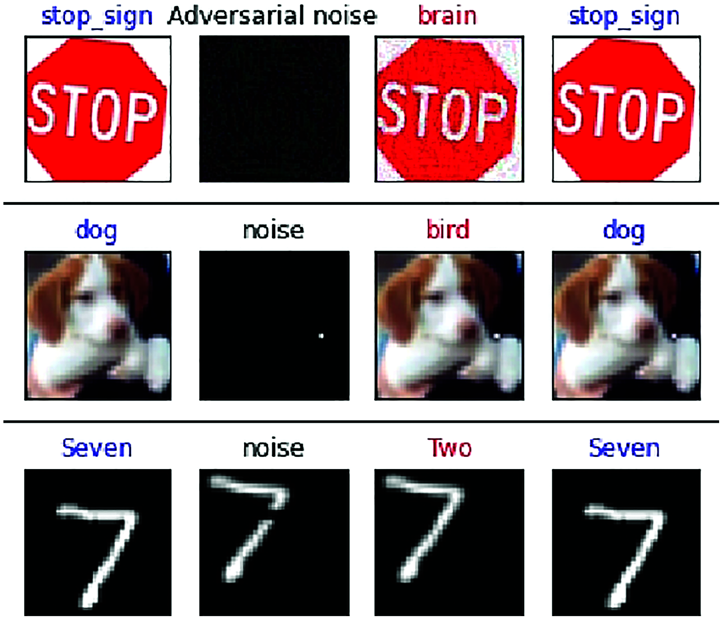
Figure 1: (a) column 1 represents the correct prediction of the model on original input images of our selected datasets. (b) column 2 represents adversarial perturbation that is added into clean input images. (c) column 3 represents the adversarial examples or images and their incorrect classification created due to three types of attacks; gradient-based attack (FGSM), score-based attacks (single pixel attack), and decision-based attacks (spatial attack). (d) column 4 represents the restored adversarial examples and their correct classification after applying our proposed method
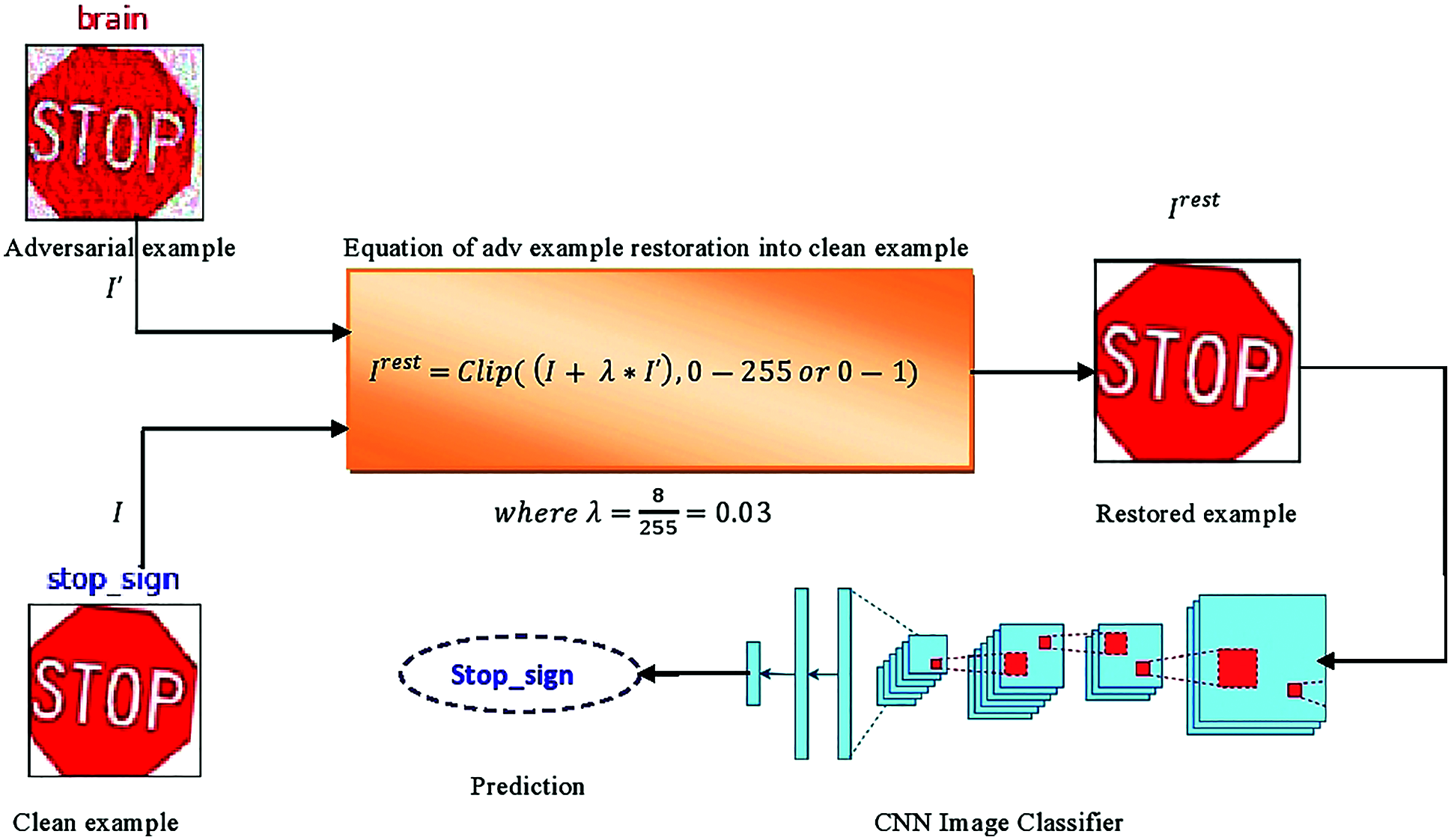
Figure 2: (a) in the first step, we have the original image with the correct label; stop-sign and its adversarial version with the incorrect label; brain (b) feed both images into the mathematical equation, which perform simple image arithmetic operations on them. (c) in this step, we get the result of our mathematical equation as a restored version of the original image and feed it into the target CNN model and check its prediction, correct, e.g., stop-sign
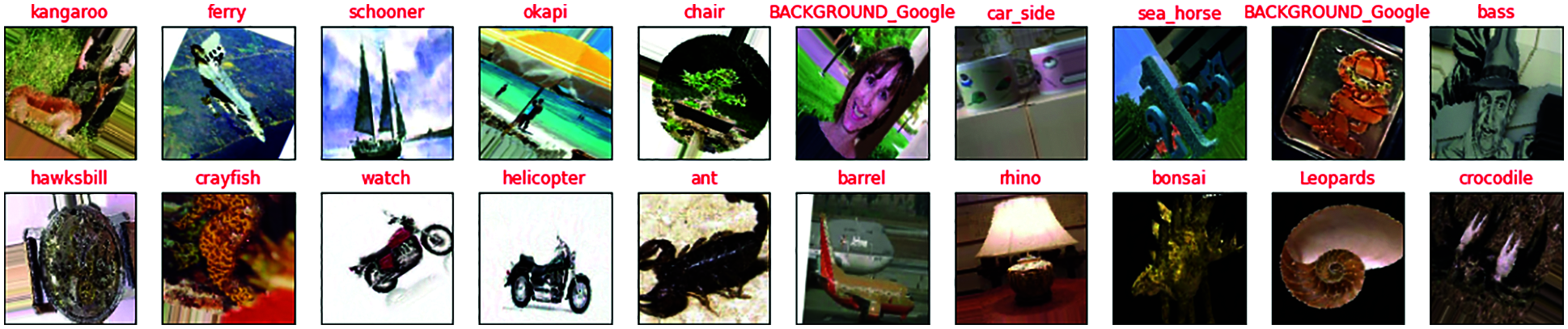
Figure 3: Adversarial examples created by BIM [36], one of the gradient-based attacks. The target model misclassifies adversarial examples; labels in red color are misclassified
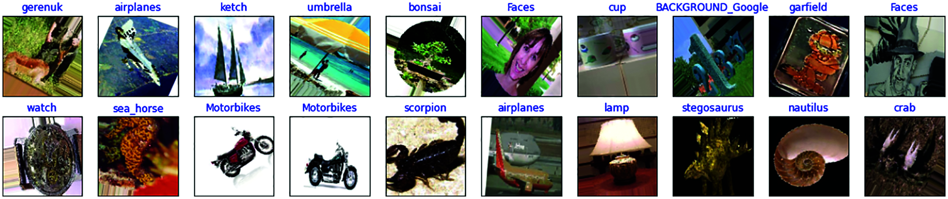
Figure 4: Results of our restoration method of adversarial examples using Eq. (12); after the restoration of adversarial example, the target model will classify correctly restored adversarial example; labels in blue colors are correctly classified

Figure 5: Adversarial example created by single pixel attack [41], one of the score-based attacks. The target model misclassifies adversarial examples; labels in red color are misclassified

Figure 6: Results of our restoration method of adversarial examples using Eq. (12); after the restoration of adversarial examples, the target model correctly classifies restored adversarial examples; labels in blue color are correctly classified

Figure 7: Adversarial examples created by spatial attack [42], one of the decision-based attacks. The target model misclassifies adversarial examples; labels in red color are misclassified
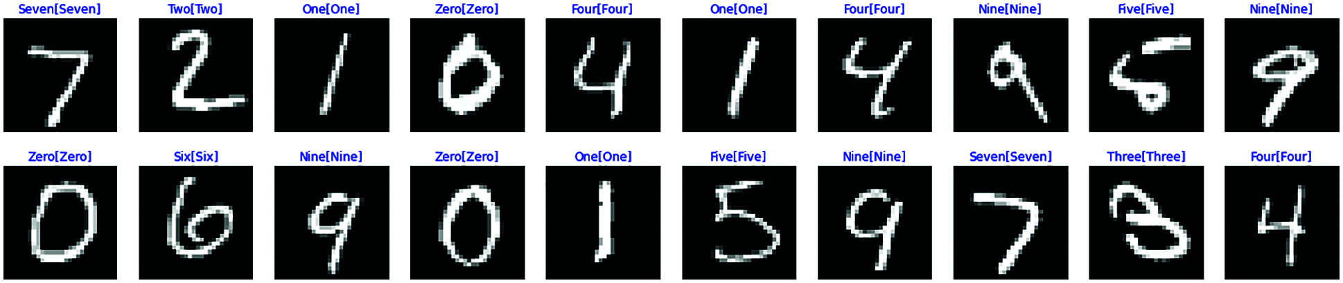
Figure 8: Results of our restoration method of adversarial examples using Eq. (12); after the restoration of adversarial examples, the target model correctly classifies restored adversarial examples; labels in blue color are correctly classified

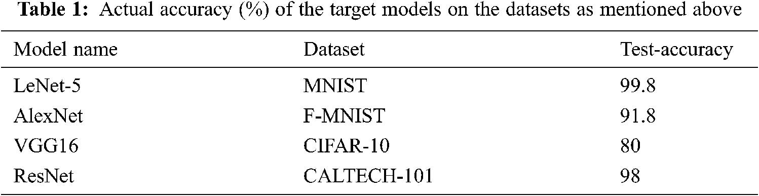
Figure 9: Actual accuracy of the target models on the selected datasets
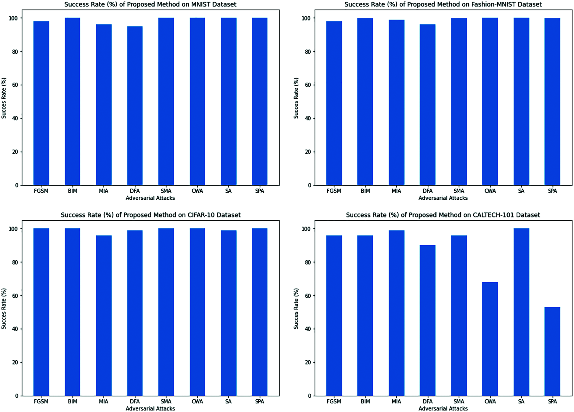
Figure 10: The success rate (%) of the proposed method against different adversarial example methods on the MNIST, F-MNIST, CIFAR-10, and CALTECH-101 datasets for LeNet, AlexNet, VGG-16, and ResNet models, respectively
The proposed mathematical method aims to restore the adversarial examples (produced by applying three types of adversarial attacks; already described in related work Section 2.1) into original or clean examples to restore or maintain the performance of a CNN model, especially an image classifier in the computer vision field. Performance means the accuracy and loss of classifiers on unseen or test images. The best classifier has high accuracy and low loss on unseen data. After the success of the adversarial attack, the classifier's accuracy is decreased. Furthermore, the loss of the classifier is increased. As a result, the classifier's performance is degraded, and the usage of the classifiers is no more required. However, in this situation, we have proposed a simple mathematical equation to restore the adversarial examples into clean or the original image so that the classifier's performance is recovered. It means the accuracy of the classifier is again high, and the loss is again low. We do not need any detector method for detecting the adversarial noise or type of adversarial attack because our proposed method will start its work after a successful adversarial attack, which can be of any attack. A successful attack means an image classifier like a CNN classifier is misclassified test images now, but these images are correctly classified before the adversarial attack.
Suppose that f is an image classifier based on CNN's architecture, I is the original input image fed to be classification and l is the original label of the input image I such that.
After the adversarial attack on f, an adversarial example I′ is created, then the Eq. (10) will become;
where I′ is the adversarial example that is slightly different from the original image I but misclassified by the classifier f. Note that the attacker is free to attack in any way, like gradient-based (FGSM, BIM), score-based attack (Single Pixel Attack), or decision boundary attack (Spatial Attack). The mathematical form of our proposed method is given by:
Here IRest is the restored image, I is the original input image, I′ is an adversarial example, l is the original label which is restored after applying Eq. (12),
Now we understand the working of our proposed method or Eq. (12) with a simple numerical example, which is given below:
Before Perturbation:
The score of category 1:
After perturbation:
The score of category 1:
The score changed from 5% to 88%.
Now we apply our proposed method or Eq. (12) to restore the prediction: Irest = x + λ*x′
Again check the probability on restored data:
Hence, the probability is restored from dog to cat again.
Also, we present some visual results which are produced in our experimental settings, shown in Figs. 3–8 for datasets caltech-101, cifar10 and mnist.
The datasets which we have used in the experimental setup are as under:
The MNIST dataset contains a total of 70000 grayscale images of handwritten digits from 0 to 9. The dimension of the images is 28 × 28. We have selected 60000 images for training the model and 10000 images for testing the model.
Fashion-MNIST also consists of 70000 greyscale images with dimensions 28 × 28 of categories belonging to clothes and shows like T-shirts, Trousers, pullovers, Dress, Coat, Sandal, shirts, sneakers, Bag, or Ankle boot. We have split 60000 images for training and 10000 for testing purposes.
In the CIFAR-10 dataset, there are 60000 thousand RGB images of different animals and vehicles like airplanes, automobiles, birds, cats, deer, dogs, frogs, horses, ships, and trucks. We have used 50000 thousand images for training and 10000 thousand for testing purposes.
This dataset has 8677 images in RGB format of 101 categories of different objects, e.g., elephant, bicycle, scooter, stop-signal. We have divided the images for training and testing purposes in the ratio of 70:30 percent.
4.5 Training Target CNN's Models
We have to use the LeNet-5 model for MNIST, AlexNet for FASHION-MNIST, VGG16 for CIFAR-10; and ResNet for CALTECH-101 dataset and thier test accuracies are shown in Tab. 1 and in Fig. 9.
We are presented the success rate of our proposed method (Eq. 12) against different adversarial attacks which are described in related work section 2.1. The results are shown in Tab. 2 and Fig. 10.
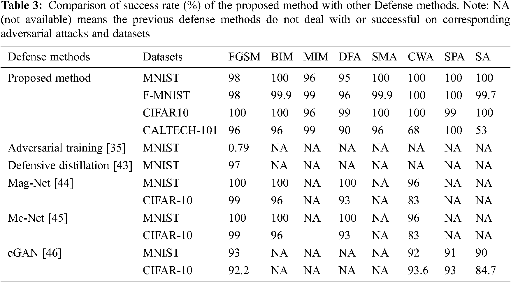
4.6 Comparison with Other Defense Methods
We present a comparison of the success rate (%) of our proposed defense method with the success rate of previous methods that are well published and discussed in our related work sections. It also shows that our method defends all three types of adversarial attacks while previous methods do not defend all attacks. We have also used four datasets, but the other methods mostly used one or two datasets only. The comparison results are given in Tab. 3.
In this work, we present a simple and computationally fast method for reconstructing perturbed images due to different types of adversarial attacks (gradient-based attacks, score-based attacks, and decision-based attacks). The proposed method recovers the performance of a model that gets badly affected by different adversarial attacks. Therefore, we claim that our method is universal because it recovers all types of adversarial examples. Our method of restoration of adversarial examples is a single-step method with low computational complexity. It is not an iterative method and only needs the original input image and an adversarial image to get back the correct intensity pattern for the correct classification of a deep learning model CNN in the computer vision field. Our experiments and their results show that our proposed method is better than the previous state-of-the-art method.

Funding Statement: The author received no specific funding for this study.
Conflicts of Interest: The authors declare that they have no conflicts of interest to report regarding the present study.
1. I. Krizhevsky, A. Sutskever and G. Hinton, “Imagenet classification with deep convolutional neural networks,” Advances in Neural Information Processing Systems, vol. 50, no. 2, pp. 1097–1105, 2012. [Google Scholar]
2. Y. LeCun, B. Boser, J. S. Denker, D. Henderson, R. E. Howard et al., “Backpropagation applied to handwritten zip code recognition,” Neural Computation, vol. 10, no. 4, pp. 541–551, 1989. [Google Scholar]
3. J. Deng, W. Dong, R. Socher, L. J. Li, K. Li et al. “Imagenet: A large-scale hierarchical image database,” in Proc. of IEEE Conf. on Computer Vision and Pattern Recognition, Miami Beach, FL, USA, pp. 248–255, 2009. [Google Scholar]
4. B. Esteva, R. Kuprel, A. Novoa, J. Ko, S. M. Swetter et al., “Dermatologist-level classification of skin cancer with deep neural networks,” Nature, vol. 542, no. 8, pp. 115–118, 2017. [Google Scholar]
5. Z. Giancarlo, M. Karim and A. Menshawy, In Deep Learning with TensorFlow, Packt Publishing Ltd, Birmingham, UK, 2017. [Google Scholar]
6. D. Silver, J. Schrittwieser, K. Simonyan, I. Antonoglou, A. Huang et al., “Mastering the game of go without human knowledge,” Nature, vol. 550, no. 7676, pp. 354–359, 2017. [Google Scholar]
7. K. He, X. Zhang, S. Ren and J. Sun, “Deep residual learning for image recognition,” in Proc. of the IEEE Conf. on Computer Vision and Pattern Recognition, Las Vagas, NY, USA, pp. 770–778, 2016. [Google Scholar]
8. C. Szegedy, V. Vincent, S. Ioffe, J. Shlens and Z. Wojna, “Rethinking the inception architecture for computer vision,” in Proc. of the IEEE Conf. on Computer Vision and Pattern Recognition, Las Vagas, NY, USA, pp. 2818–282, 2016. [Google Scholar]
9. G. Huang, Z. Liu, K. Q. Weinberge and L. Maaten, “Densely connected convolutional networks,” in arXiv preprint arXiv:1608.06993, 2016. [Google Scholar]
10. L. Vedaldi and K. Lenc, “Matconvnet–convolutional neural networks for MATLAB,” in Proc. of the ACM Int. Conf. on Multimedia, Brisbane, Australia, 2015. [Google Scholar]
11. J. Yangqing, E. Shelhamer, J. Donahue, S. Karayev, J. Long et al., “Caffe: Convolutional architecture for fast feature embedding,” in arXiv preprint arXiv:1408.5093, 2014. [Google Scholar]
12. M. Abadi, A. Agarwal, P. Barham, E. Brevdo and Z. Chen, “Tensorflow: Large-scale machine learning on heterogeneous systems,” Software Available from Tensorflow.org, in arXiv preprint arXiv:1603.04467, 2015. [Google Scholar]
13. C. Kai, H. Zhu, L. Yan and J. Wang, “A survey on adversarial examples in deep learning,” Journal on Big Data, Tech Science Press, vol. 2, no. 2, pp. 71, 2020. [Google Scholar]
14. M. Najafabadi, F. Villanustre, T. M. Khoshgoftaar, N. Seliya, R. Wald et al., “Deep learning applications and challenges in big data analytics,” Journal of Big Data, vol. 2, no. 1, pp. 110–118, 2015. [Google Scholar]
15. N. Papernot, P. McDaniel, A. Sinha and M. Wellman, “Towards the science of security and privacy in machine learning,” in arXiv preprint arXiv:1611.03814, 2016. [Google Scholar]
16. K. Grosse, N. Papernot, P. Manoharan, M. Backes and P. Daniel, “Adversarial examples for malware detection,” in Pro. of European Symposium on Research in Computer Security, Oslo, Norway, pp. 62–79, 2017. [Google Scholar]
17. M. Volodymyr, K. Kavukcuoglu, D. Silver, A. A. Rusu, J. Veness et al., “Human-level control through deep reinforcement learning,” Nature, vol. 518, no. 7540, pp. 529–533, 2015. [Google Scholar]
18. A. Giusti, J. Guzzi, D. C. Ciresan, F. He, J. P. Rodriguez et al., “A machine learning approach to visual perception of forest trails for mobile robots,” IEEE Robotics and Automation Letters, vol. 1, no. 2, pp. 661–667, 2016. [Google Scholar]
19. G. Hinton, L. Deng, D. Yu, G. E. Dahl, A. R. Mohamed et al., “Deep neural networks for acoustic modeling in speech recognition,” The Shared Views of Four Research Groups, IEEE Signal Processing Magazine, vol. 29, no. 6, pp. 82–97, 2012. [Google Scholar]
20. Z. Jiliang and C. Li, “Adversarial examples: Opportunities and challenges,” IEEE Transactions on Neural Networks and Learning Systems, vol. 31, no. 7, pp. 2578–2593, 2019. [Google Scholar]
21. I. Goodfellow, J. Shlens and C. Szegedy, “Explaining and harnessing adversarial examples,” in arXiv preprint arXiv:1412.6572, 2014. [Google Scholar]
22. A. M. Nguyen, J. Yosinski and J. Clune, “Deep neural networks are easily fooled: High confidence predictions for unrecognizable images,” in Proc. of IEEE Conf. on Computer Vision and Pattern Recognition, CVPR 2015, Boston, USA, pp. 427–436, 2015. [Google Scholar]
23. M. Sharif, S. Bhagavatula, L. Bauer and M. Reiter, “Accessorize to a crime: Real and stealthy attacks on state-of-the-art face recognition,” in Proc. of the 2016 ACM SIGSAC Conf. on Computer and Communications Security, Vienna, Austria, pp. 1528–1540, 2016. [Google Scholar]
24. C. Szegedy, W. Zaremba, I. Sutskever, J. Bruna, D. Erhan et al., “Intriguing properties of neural networks,” in arXiv preprint arXiv:1312.6199, 2013. [Google Scholar]
25. A. Fawzi and P. Frossard, “Analysis of classifiers’ robustness to adversarial perturbations,” in arXiv preprint arXiv:1502.02590, 2015. [Google Scholar]
26. A. Kurakin, I. Goodfellow and S. Bengio, “Adversarial machine learning at scale,” in arXiv preprint arXiv:1611.01236, 2016. [Google Scholar]
27. N. Papernot and P. McDaniel, “On the effectiveness of defensive distillation,” in arXiv preprint arXiv:1607.05113, 2016. [Google Scholar]
28. A. Rozsa, M. Günther and T. E. Boult, “Towards robust deep neural networks with BANG,” in arXiv preprint arXiv:1612.00138, 2016. [Google Scholar]
29. M. A. Torkamani, “Robust large margin approaches for machine learning in adversarial settings,” PhD thesis, University of Oregon, 2016. [Google Scholar]
30. J. Sokolic, R. Giryes, G. Sapiro and M. R. Rodrigues, “Robust large margin deep neural networks,” in arXiv preprint arXiv:1605.08254, 2016. [Google Scholar]
31. F. Tramer, N. Papernot, I. J. Goodfellow, D. Boneh and P. D. McDaniel, “The space of transferable adversarial examples,” in arXiv preprint arXiv:1704.03453, 2017. [Google Scholar]
32. A. M. Nguyen, J. Yosinski and J. Clune, “Deep neural networks are easily fooled: high confidence predictions for unrecognizable images,” in Proc. of IEEE Conf. on Computer Vision and Pattern Recognition, CVPR 2015, Boston, USA, pp. 427–436, 2015. [Google Scholar]
33. M. Sharif, S. Bhagavatula, L. Bauer and M. K. Reiter, “Accessorize to a crime: real and stealthy attacks on state-of-the-art face recognition,” in Proc. of the 2016 ACM SIGSAC Conf. on Computer and Communications Security, Vienna, Austria, pp. 1528–1540, 2016. [Google Scholar]
34. S. Mohsen, M. Dezfooli, A. Fawzi and P. Frossard, “Deepfool: a simple and accurate method to fool deep neural networks,” in Proc. 2016 IEEE Conf. on Computer Vision and Pattern Recognition, CVPR 2016, Las Vegas, NV, USA, pp. 2574–2582, 2016. [Google Scholar]
35. J. Goodfellow, J. Shlens and C. Szegedy, “Explaining and harnessing adversarial examples,” in Proc. ICML, Beijing, China, pp. 278–293, 2014. [Google Scholar]
36. A. Kurakin, I. Goodfellow and S. Bengio, “Adversarial examples in the physical world,” in Proc. ICLR, Toulon, France, pp. 1726–1738, 2016. [Google Scholar]
37. D. Yinpeng, F. Liao, T. Pang, H. Su, J. Zhu et al., “Boosting adversarial attacks with momentum,” in Proc. of the IEEE Conf. on Computer Vision and Pattern Recognition, Salt Lake City, UT, USA, pp. 9185–9193, 2018. [Google Scholar]
38. M. Dezfooli, S. Mohsen, A. Fawzi and P. Frossard, “Deepfool: a simple and accurate method to fool deep neural networks,” in Proc. of the IEEE Conf. on Computer Vision and Pattern Recognition, Las Vegas, NV, USA, pp. 2574–2582, 2016. [Google Scholar]
39. P. Nicolas, P. McDaniel, S. Jha, M. Fredrikson, Z. B. Celik et al., “The limitations of deep learning in adversarial settings,” in Proc. 2016 IEEE European Symposium on Security and Privacy (EuroS&PSaarbrucken, Germany, pp. 372–387, 2016. [Google Scholar]
40. C. Nicholas and D. Wagner, “Towards evaluating the robustness of neural networks,” in 2017 IEEE Symposium on Security and Privacy (SPParis, France, pp. 39–57, 2017. [Google Scholar]
41. N. Nina and S. P. Kasiviswanathan, “Simple black-box adversarial perturbations for deep networks,” in arXiv preprint arXiv:1612.06299, 2016. [Google Scholar]
42. E. Logan, B. Tran, D. Tsipras, L. Schmidt and A. Madry, “A rotation and a translation suffice: Fooling cnns with simple transformations,” in arXiv preprint arXiv:1712.02779, 2018. [Google Scholar]
43. P. Nicolas, P. McDaniel, X. Wu, S. Jha and A. Swami, “Distillation as a defense to adversarial perturbations against deep neural networks,” in Proc. of 2016 IEEE Symposium on Security and Privacy (SPSan Jose, California, USA, pp. 582–597, 2016. [Google Scholar]
44. M. Dongyu and H. Chen, “Magnet: A two-pronged defense against adversarial examples,” in Proc. of the 2017 ACM SIGSAC Conf. on Computer and Communications Security, Dallas,Texas,USA, pp. 135–147, 2017. [Google Scholar]
45. Y. Yuzhe, G. Zhang, D. Katabi and Z. Xu, “Me-net: Towards effective adversarial robustness with matrix estimation,” in arXiv preprint arXiv:1905.11971, 2019. [Google Scholar]
46. C. Xie, J. Wang and Z. Zhang, “The defense of adversarial example with conditional generative adversarial networks,” Security and Communication Networks, vol. 1, no. 3, pp. 140–152, 2020. [Google Scholar]
 | This work is licensed under a Creative Commons Attribution 4.0 International License, which permits unrestricted use, distribution, and reproduction in any medium, provided the original work is properly cited. |