DOI:10.32604/iasc.2022.021461
| Intelligent Automation & Soft Computing DOI:10.32604/iasc.2022.021461 | |
| Article |
A Mathematical Optimization Model for Maintenance Planning of School Buildings
1Department of Civil Engineering, Kish International Branch, Islamic Azad University, Kish Island, Iran
2Department of Civil Engineering, Roudehen Branch, Islamic Azad University, Roudehen, Iran
3Department of Civil Engineering, Safadasht Branch, Islamic Azad University, Safadasht, Iran
*Corresponding Author: Babak Aminnejad. Email: aminnejad@riau.ac.ir
Received: 03 July 2021; Accepted: 07 August 2021
Abstract: This article presents a methodology to optimize the maintenance planning model and minimize the total maintenance costs of a typical school building. It makes an effort to provide a maintenance schedule, focusing on maintenance costs. In the allocation of operations to the school equipment, the parameter of its age was also taken into account. A mathematical optimization model to minimize the school maintenance cost in a three-year period was provided in the GAMS software with CPLEX solver. Finally, the optimum architecture of the Perceptron multi-layer neural network was used to predict the schedule of equipment operations and maintenance costs. The Multi-layer Perceptron (MLP) optimum neural network results, with minor Mean Squared Error (MSE) and Root Mean Squared Error (RMSE), indicated that the proposed model was capable of predicting the schools’ maintenance costs with high accuracy. According to the results, the school's maintenance cost for the intended three-year period based on the Weibull distribution was equal to 15361 currency units per hour, in which the “heating and cooling system” has the highest contribution. Hence, accurate and definite planning can prevent damages to such equipment, while saving the school's maintenance costs.
Keywords: Mathematical modelling; maintenance planning; educational buildings; cost optimization; neural network
Maintenance of educational building assets is an important tool not only for the wellness of students and other users, but also for school life cycle maximization and minimization of maintenance costs [1]. It takes a continuous operation to keep the school buildings, furniture, and equipment in the best form for normal use [2–8]. In fact, the management of building maintenance means how the maintenance process should be financially and technologically organized to deal with the issue of building maintenance [9].
The integrated production and maintenance planning models have been seriously studied since the early 80 s. Over time, integrated models have been separated according to their maintenance methods (predictive/corrective and periodic/non-periodic). The non-periodic maintenance in integrated models has been less studied since, in such conditions, the solution is tough, and usually, the branch and bound method is used to solve it. For a better understanding of the required concepts of maintenance in the next sections, a summary for each of them is provided in this section. In general, the maintenance and repair can be defined as the following: A combination of activities conducted particularly and in a usual planned way to prevent the sudden failure of machinery, equipment, and facilities is called maintenance [10–13]. The repair includes a set of activities performed on a system or tool that has failed or been disabled to return it to the ready-for-operation mode and prepare it to conduct its duties [13].
The maintenance has been created from several important classes of decision-making: 1) strategic concept and long-term maintenance, 2) medium-term planning, 3) short-term planning, and 4) control and performance indexes [14]. Important decision-making strategies evaluate maintenance in the design of system processes. They consider which type of maintenance is suitable and when it should be done. Many optimization models consider these issues and the relationship with production, which has been revealed in some cases [14]. Many studies have been conducted on maintenance planning optimization so far. The decision-making in this field is developed based on multi-criteria decision-making models, such as the Analytic Hierarchy Process (AHP), Technique for Order of Preference by Similarity to Ideal Solution (TOPSIS), or multi-objective optimization models, in the framework of operations research. Condition-based planning is one of the newest and best maintenance planning methods. Therefore, this research has employed condition-based planning. In the following, we review the literature in this field. Badıa et al. [15] proposed an inspection procedure for failure detection in a single-unit system. In this system, different types of failures are possible, and the probability of each failure depends on its type. Lam et al. [16] suggested a condition-based maintenance planning model for a system exposed to failure. In this model, the failure could be detected through a 100% inspection. Furthermore, a particular relationship between the inspection and failure probability, as well as an incorrect alarm, was considered in this research. Zequeira et al. [17] developed the previously developed models by dividing the inspection into the three following classes:
(a) Complete inspection (faultless inspection for all systems)
(b) Partial inspection (only error type 1)
(c) Incomplete inspection (only detection of error type 2) that may also provide false positive results for other types of failures.
He et al. [18] developed a special form of the model suggested by Zequeira and Bérenguer. In this mode, the research was carried out without partial inspections. Generally, the partial inspection-based models are very limited due to their complexity in mathematical modeling. In this regard, Noortwijk et al. [19] conducted a research review of the maintenance models based on the gamma process in the incomplete inspection. Similar models were also developed by Ye et al. [20] in the incomplete inspection. Si et al. [21] performed condition-based mathematical modeling to find the optimum number of inspection times, replacement threshold, and complete reconstruction of systems to minimize the total implementation cost. According to this model, the following two measures should be taken to achieve the optimum plan:
(a) Determining whether the system requires preventive or corrective maintenance.
(b) Determining the optimum inspection time until the next inspection
In another study, Fouladirad et al. [22] extended the previously developed model, by considering dynamism in the system's failure rate. Their paper proposed one of the newest approaches to condition-based maintenance modeling. There are also plenty of research papers on Machine learning [23], optimization [24–30] and mathematical modeling of different systems [31–40].
The current paper however, proposes a mathematical model for schools’ maintenance planning to minimize the total maintenance cost. For this purpose, after providing the mathematical model, the essential indexes and equipment of a sample school are used along with a neural network to provide cost prediction for a three-year planning horizon. The main novelties of this work are presenting an optimum maintenance plan for the school buildings with the minimum cost, future cost prediction ability and consideration of the age of school's equipment. To the best of our knowledge, this is the first time that these issues are addressed.
The considered domain in this paper is a school with the equipment of cooling and heating systems, educational and laboratory equipment, and lavatories. In order to conduct the maintenance and repair of the equipment, a schedule for the maintenance and a schedule for the preventive repair of equipment are required. The ages of equipment (total working hours of each equipment) are different, but all known. The maintenance operations can be planned for various pieces of equipment with different ages and costs. It is clear that their maintenance costs have a direct relationship with their ages. This research work proposes a mathematical planning model to provide an equipment maintenance schedule while minimizing the total maintenance costs. In fact, the maintenance operations schedule in the three-year period which yields to the minimum cost is obtained via an optimization algorithm. Then, based on the available data for the three-year period, the values of cost and maintenance operations schedule for the fourth and fifth years in the intended school are estimated using the artificial neural network.
In this section, the problem assumptions, model components, and the main model are expressed.
• This paper employs the two policies of emergency (unplanned) maintenance and preventive maintenance.
• The equipment failure rate is considered constant based on the Weibull distribution function.
• The costs of unplanned (emergency) maintenance are more than those of preventive maintenance.
• The planning is provided in the framework of a particular time horizon. (The problem is divided into n periods.)
• The age ranges are considered constant (each equipment piece's age is classified with respect to the ranges).
It is assumed that the age density of the equipment is in the form of Weibull function as follows:
where
Γ: Gamma function
μ: The mean of Weibull distribution
σ2: The variance of Weibull distribution
R(t): Distribution reliability
Indexes
i: Equipment No.
b: Age range No.
y: Period
c: Critical period No. (major repairs)
Parameters
Cost p (i,b,y): Cost of preventive maintenance of equipment i, age range b, period y
Cost f (i,b,y): Cost of corrective (emergency) maintenance of equipment i, age range b, period y
F(L(i)): Accumulative failure distribution function of equipment i
MTTR f: Mean time required for repair or exchange of failure
MTTR_b: Mean time required for preventive maintenance
tf: Period between two emergency failures
R(y): Required repair time in period y
α(i): Scale parameter of Weibull distribution for equipment i
β: Shape parameter of Weibull distribution
A(i,y): The available time for equipment i in period y
M(i,b): The maximum available time for equipment i in period b
EF(i): Cost of major repair for equipment i
Decision variable
X(i,b,y): The planned working time for equipment i in age range b in period (year) y
L(i): Period of performing preventive maintenance for equipment i
Y(i,b,y): If equipment i in the age range b uses the entire available time of period y, one; otherwise, zero
Yc(i,b,y): If equipment i in the age range b and period y is subjected to a major repair, one; otherwise, zero
H(i,y): The accumulated use hours of equipment i in period y, which is equal to equipment age for y = 0 and accumulated used hours for y > 0.
The objective function is determined according to the criterion of equipment maintenance in unit time. The cost is always an important and effective factor in selecting the maintenance policies in organizations. While investigating maintenance policies, most maintenance researchers and engineers have sought a policy to minimize it. Therefore, it has always been a determining factor in organizations. Eq. (4) demonstrates the preventive maintenance cost. In this equation, if L(i) is the preventive maintenance period for equipment i, UEC(L(i)) equals the preventive maintenance cost rate in the L(i)th preventive maintenance period of equipment i. In fact, it is assumed that each L(i) time unit spent is allocated to perform preventive maintenance on it, and L(i) is the decision variable.
The numerator of the fraction in Eq. (4) is equal to the total expected cost, and its denominator denotes the expected cycle time. In this equation, the accumulative distribution function of equipment i is denoted with F(L(i)). Therefore, by substituting for the Weibull distribution information in Eq. (4) and calculating the total costs for all equipment pieces in the age ranges and the entire period, the objective function is as follows:
The model constraints are as the following:
In the equations above i_max, b_max, y_max, and MM are the total number of equipment pieces, the total number of age ranges, total number of periods, and a relatively large number.
The objective function minimizes all cycles’ maintenance cost for the favorable function of equipment and optimum maintenance intervals. The nominator of the fraction in the objective function is the emergency and preventive maintenance cost for their occurrence probability, and the denominator is equal to the expected length of each cycle. Constraint (7) guarantees that the total time allocated to each equipment piece in all age ranges does not exceed the access time. Constraint (8) limits the model so that the total time allocated to each equipment piece in each age range in all periods does not exceed the maximum available time in that age range. Constraint (9) shows that the total time allocated in all age ranges for each equipment piece in each period equals the difference between cumulative time in two successive periods. Constraints (10) and (11) guarantee that each equipment piece receives time in its age range, and unless the previous age range is not filled, the next range does not receive time. Constraint (12) satisfies the production time in each period in the studied industry. Constraints (13) and (14) show the major repair time for a critical range. Constraints (15) and (16) indicate the positivity and type of variables.
In this section, in order to evaluate the model and determine the value of the objective function, coding in the GAMS software on a system with a Core i5 processor and 8 GB Ram was conducted. The used solver was the CPLEX algorithm. The properties of the studied school are listed in Tab. 1. Parameters values are obtained from two sources: firstly, by collecting information from a questionnaire among 1,000 teachers and school principals and selecting 278 people using Morgan sampling. Cronbach's alpha was used to calculate the reliability of the questionnaire. Using Spss22 software, the necessary calculations were performed and it was found that the prepared questionnaire has a reliability of 89.6%, which is an acceptable value. Secondly, through the information contained in the instructions released by the Organization for Development, Renovation and Equipping schools of Iran. By referring to this instruction and inquiring about the current price of each item, the relevant costs can be obtained. We use unitless currency in this research to makes it more general.
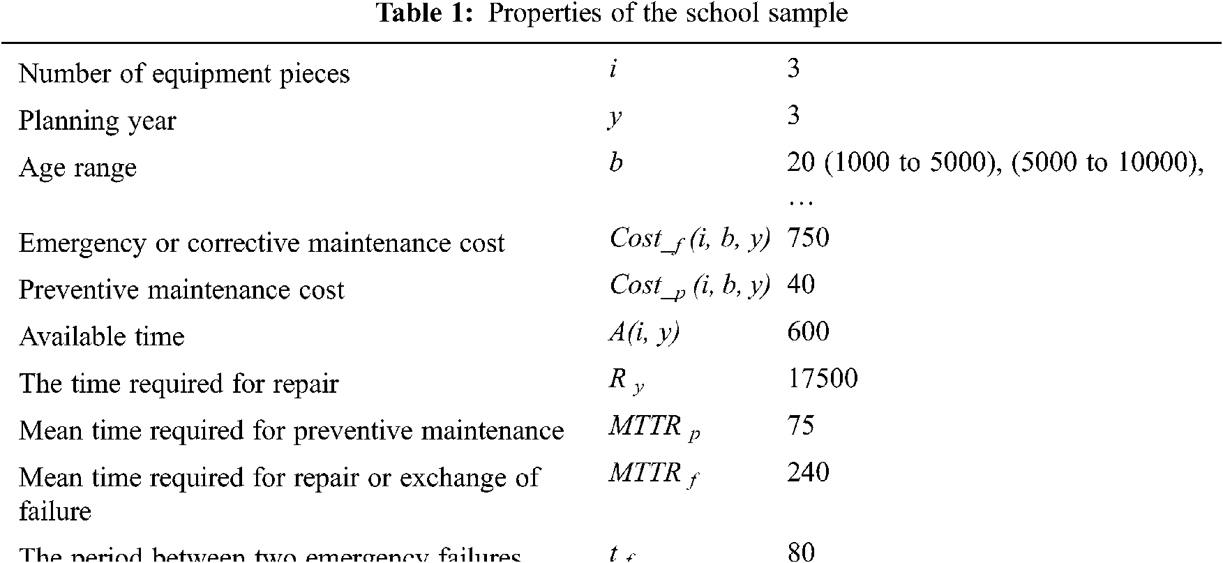
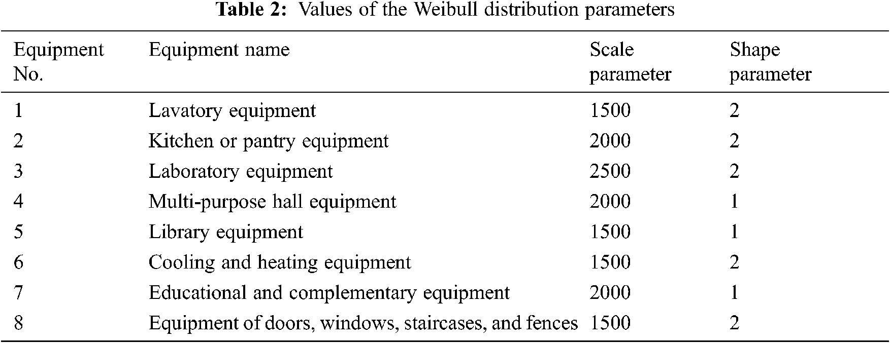
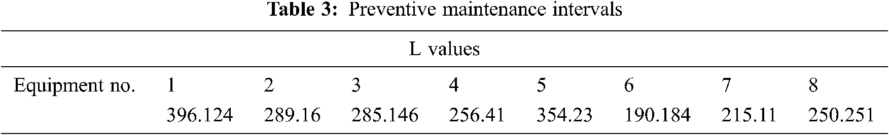
Tabs. 2 and 3 provide the parameters of Weibull distribution and preventive maintenance intervals, respectively.
Using the data given in the previous sections, results are provided in two subsections. Firstly, using the GAMS software, the optimal value of the objective function, i.e., the minimum cost of the school maintenance operations schedule in the three-year period (X(i,b,y)), is determined. Then, a data set is prepared for the cost and schedule of the operations by changing the values of the initial data, and the values of cost and X(i,b,y) for the fourth and fifth years in the intended school are estimated using the artificial neural network in the MATLAB software.
5.1 Results of the Accurate Solution of the Model
Tab. 4 provides the equipment operations schedule values in various range numbers for each studied three-years time span, based on which the lowest maintenance cost can be determined.
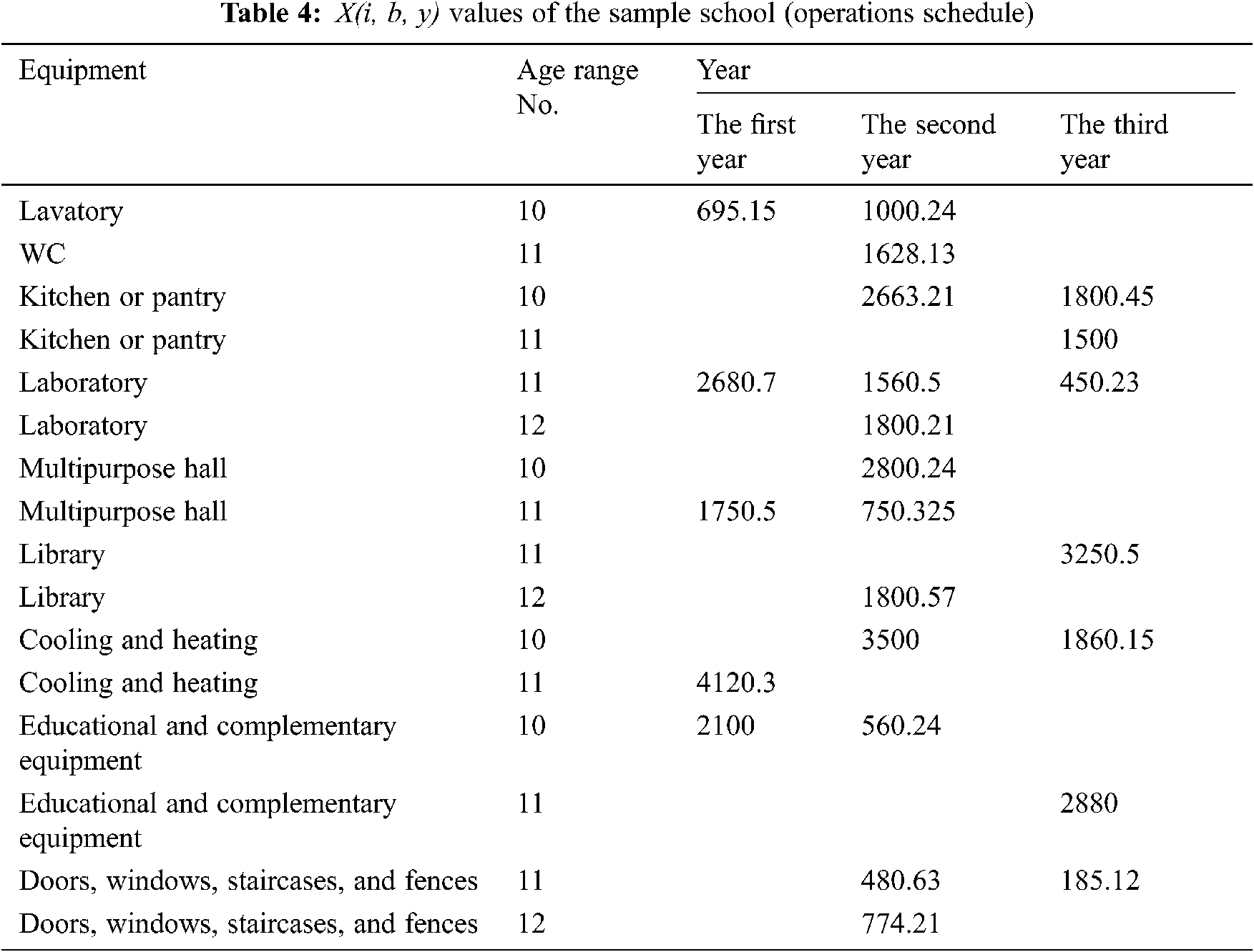
According to the schedule suggested for the equipment, the school's maintenance cost for the intended three-year period is equal to 15361 currency units per hour.
5.2 Results of the Two-Year Prediction (The Fourth and Fifth Years)
Before using the neural network, its different learning functions were used to determine which function had the best performance. The table below lists the correlation results of each of the learning functions. In order to determine the performance of the best learning function, the number of hidden layers and the number of neurons were both considered 10. It is worth mentioning that in this step, 70% of the data were used in the learning stage, 15% were used in the testing stage, and another 15% were used in the verification (assessment) stage. Accordingly, the best correlation values for each learning function were determined, based on which the correlation of values could be determined separately for each test. The results of the different functions are given in Tab. 5.
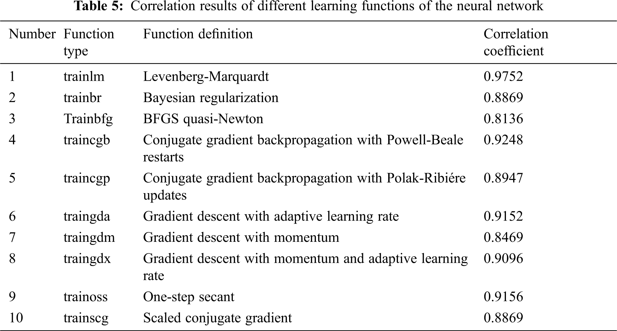
As can be seen, among the functions above, the function trainlm had the highest correlation. Therefore, it was used for data learning. In the next step, the network model was evaluated and developed based on the number of layers and neurons. The two commonly used types of the neural network, i.e., the Multi-layer Perceptron (MLP) and Radial Basis Function (RBF), were employed to assess the neural network. The best architectures of the neural networks MLP and RBF are provided in Tabs. 6 and 7, respectively.

The number of layers and neurons is of crucial importance in the MLP neural network so that an increase or decrease in them can influence the network performance.
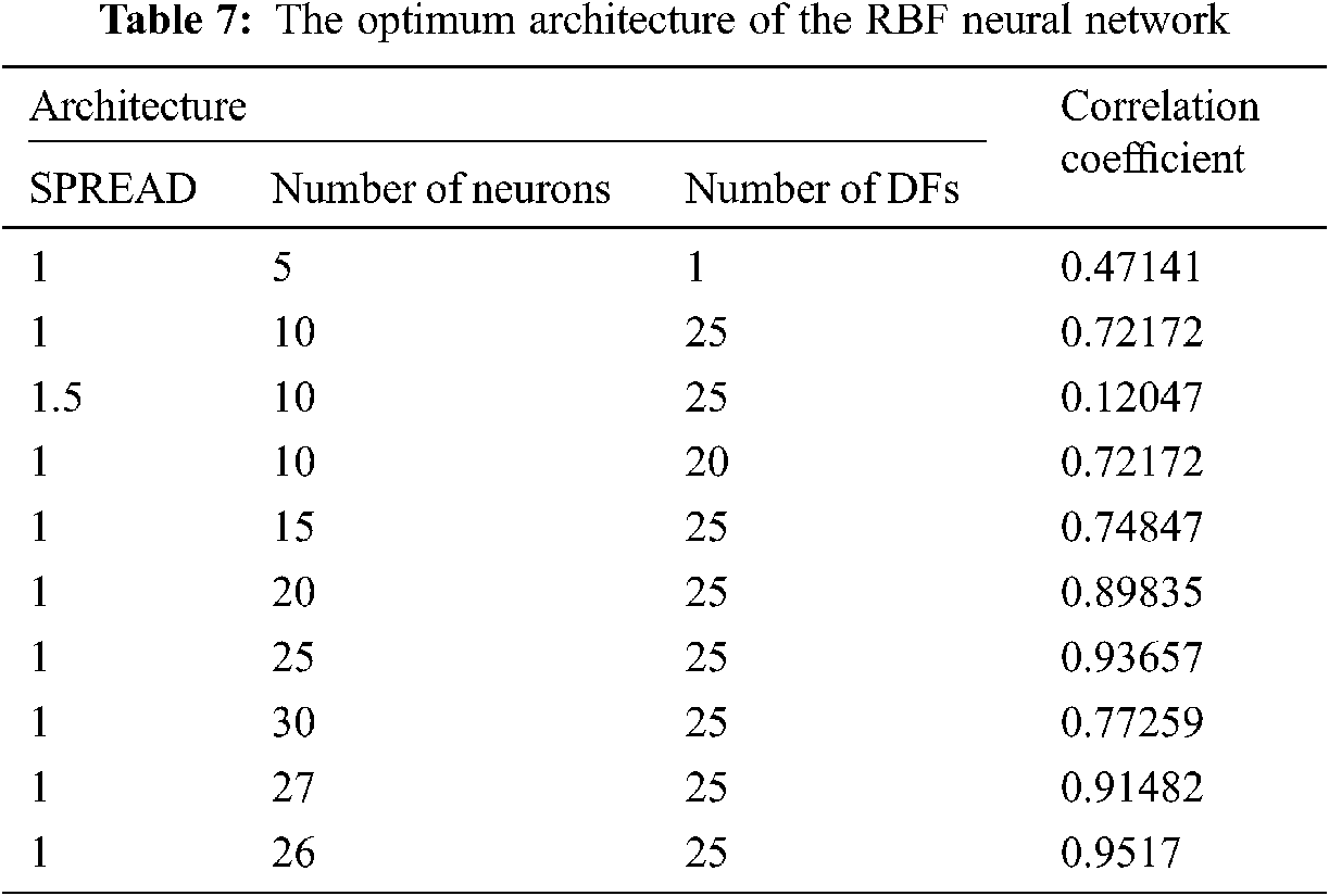
In the RBF neural network, the most important parameters affecting the network performance are the SPREAD, number of neurons, and the number of neurons located between the displays (DF). Thus, before modeling each of the membranes using the RBF neural network, it is essential to determine the favorable number of neurons and DFs for modelling, as shown in Tab. 7.
Fig. 1 illustrates the correlation coefficient variations for each of the two neural networks based on their optimum architectures.
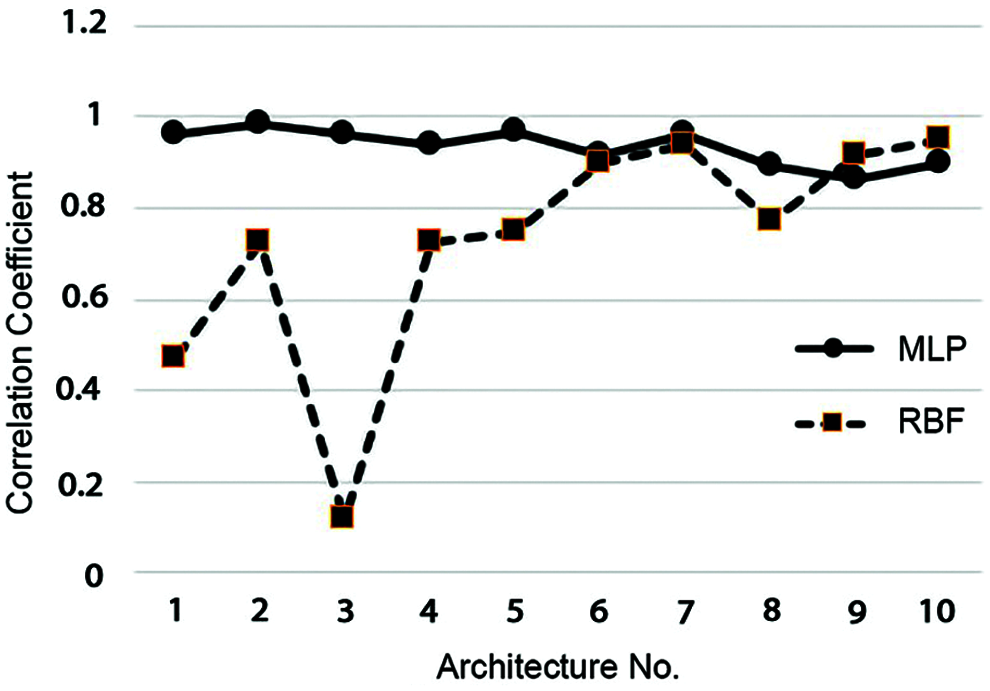
Figure 1: A comparison between the performances of different architectures of MLP and RBF neural networks in terms of correlation
As can be seen, the MLP neural network's optimum architecture in predicting the operations schedule and maintenance cost was the second one with 10 layers and 20 neurons. Furthermore, the RBF neural network's optimum architecture was the tenth architecture with a SPREAD of 1, 26 neurons, and 25 DFs. Therefore, the model was evaluated based on the input data and the learning function of trainlm with the optimum architecture of both methods. For this purpose, the 70% learning, 15% testing, and 15% assessment data were evaluated. Figs. 2 and 3 depict the results obtained from the correlation between all data in both learning and testing stages for the MLP and RBF neural networks, respectively.
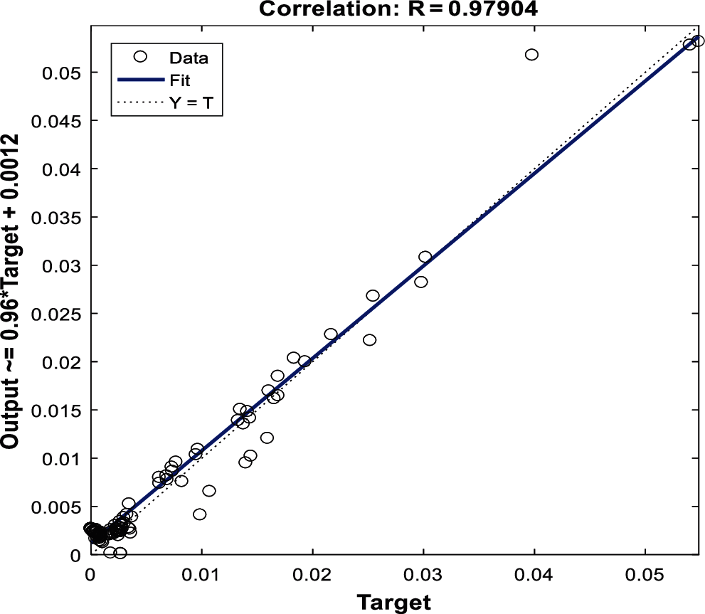
Figure 2: Data correlation curve in MLP neural network
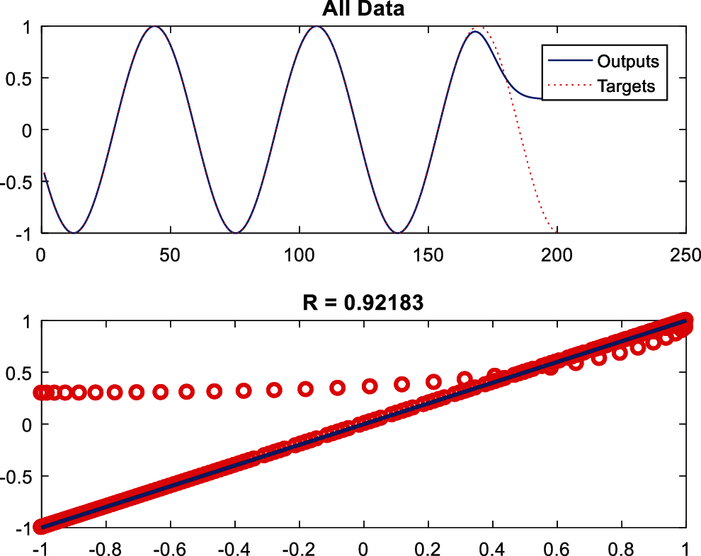
Figure 3: Data correlation curve in RBF neural network
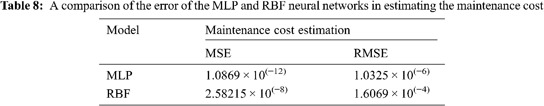
Tab. 8 compares the modelling error of both networks. As can be seen, the MLP neural network has a better performance compared to the RBF neural network.
Finally, the operations schedule and maintenance cost of the school equipment were predicted with the MLP neural network model (Tab. 9).
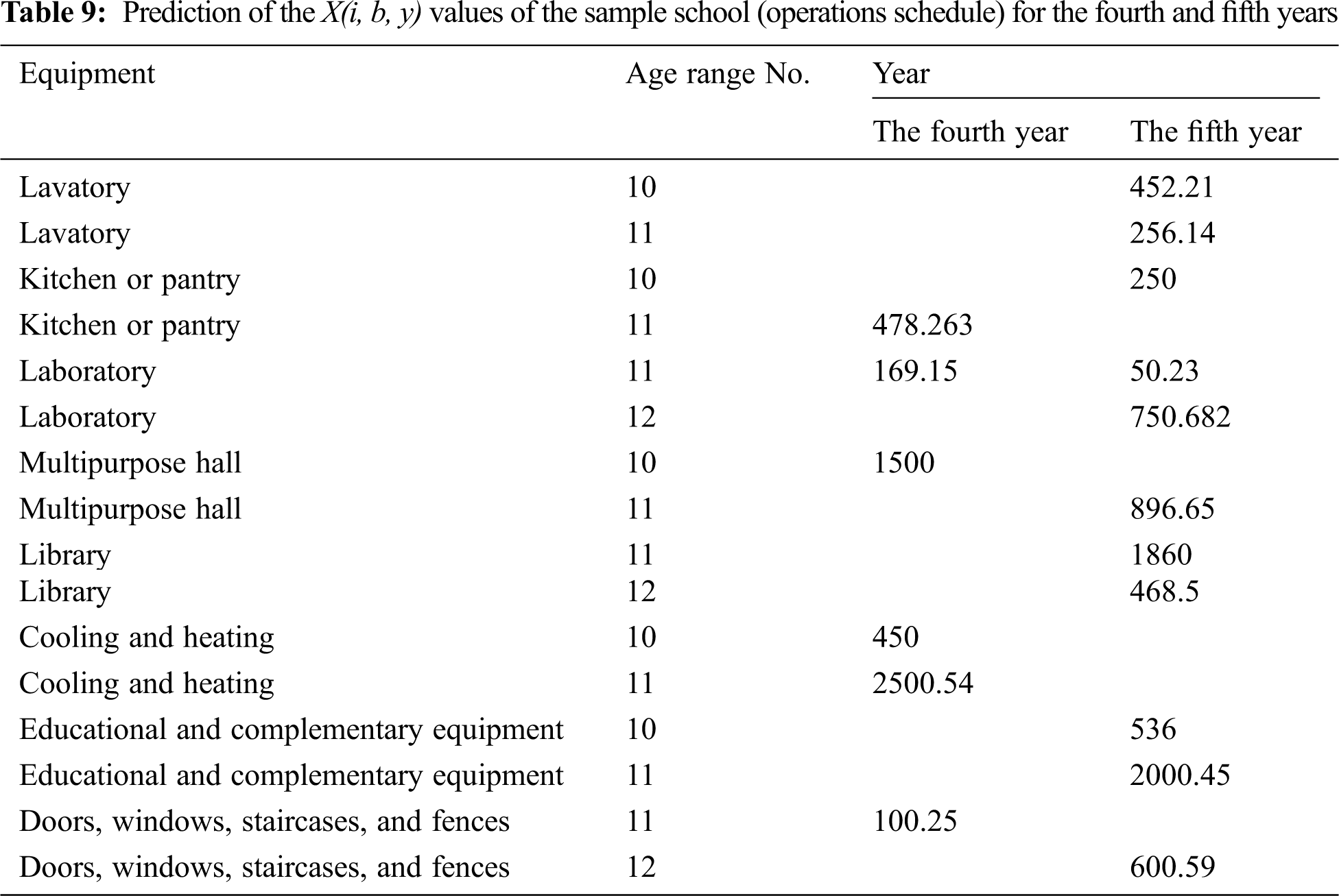
As can be seen in the table above, the maintenance cost increases with the operations schedule. Accordingly, considering the previous three-year cost, the maintenance cost for a five-year period for the intended equipment in Tab. 9 is equal to 19583 currency units per hour. Based on this planning period, it was found that after the fifth year, the maintenance and painting costs of the doors, windows, staircases, fences, and spaces of the school would rise. Moreover, in the next years, the building's costs would also grow due to the increased age and deterioration of the building.
A mathematical optimization model for the maintenance planning of schools is presented. For this purpose, a model based on the optimum preventive and corrective maintenance was designed for a sample school to reduce the school equipment's maintenance and repair costs. The results of the sample school maintenance plan were evaluated in two sections. In the first section, by modelling in the GAMS software and using the CPLEX solver, the operations schedule and maintenance cost for three different types of equipment in the school and a three-year period were investigated. In the next step, the two famous neural networks, i.e., MLP and RBF, were employed with their optimum architectures. It was found that the MLP neural network with a MSE error of 1.0869 × 10(−12) and RMSE error rate of 1.0325 × 10(−6) had better performance compared to the RBF neural network. Therefore, the fourth- and fifth-years’ operations schedule and maintenance costs were predicted using this neural network. Using this method and considering the previous three-year cost, the equipment maintenance cost for the desired five-year period was obtained 19853 currency units per hour. Hence, it can be claimed that the suggested model is capable of predicting the schools’ equipment maintenance costs with high accuracy. It was also found that among entire equipment pieces, the heating and cooling system and the laboratory equipment had higher maintenance costs, equal to almost 35% of the school's total maintenance costs. Hence, accurate and definite planning can prevent such equipment damages while saving the school's maintenance costs. This work has been conducted only for a specific period of the building's life time, so similar surveys at different time points are recommended. The assessment of the optimization results is possible through implementation of the obtained maintenance plan in practice and evaluate the costs at the end of the program. The same methodology can be used for modelling, optimization and predicting the maintenance cost of other buildings, such as residential and commercial ones to reduce their maintenance costs and increase their reliability. The technology of real-time streaming through internet of things (IOT) can be implemented for predictive maintenance in schools’ buildings and equipment. They make the scope of our future researches.
Funding Statement: The authors received no specific funding for this study.
Conflicts of Interest: The authors declare that they have no conflicts of interest to report regarding the present study.
1. A. A. Pérez, A. Vieira and A. M. Cardoso, “School buildings assets-maintenance management and organization for vertical transportation equipment,” in Proc. WCEAM, Athens, Greece, pp. 59–67, 2009. [Google Scholar]
2. L. W. Moon, “Maintenance and operation of school buildings,” Review of Educational Research, vol. 12, no. 2, pp. 228–36, 1942. [Google Scholar]
3. D. Arditi and M. Nawakorawit, “Designing building for maintenance: Designers’ perspective,” Journal of Architectural Engineering, vol. 5, no. 4, pp. 107–108, 1999. [Google Scholar]
4. O. A. Latef, M. F. Khamidi and A. Idrus, “Building maintenance management in a Malaysia university campus: A case study,” Australasian Journal of Construction Economics and Building, vol. 10, no. 2, pp. 101–114, 2010. [Google Scholar]
5. J. Douglas and B. Ransom, Understanding Building Failures, 4th ed, London, UK: Taylor and Francis, pp. 222–232, 2006. [Google Scholar]
6. W. H. Ransom, Building Failures Diagnosis and Avoidance, London, UK: E. & F. N. Spon, vol, 2, pp. 62, 1987. [Google Scholar]
7. A. G. Ahmad, “Understanding common building defects: The dilapidation survey report,” Majalah Akitek, vol. 16, no. 1, pp. 19–21, 2004. [Google Scholar]
8. A. Z. A. Akasah and B. M. Alias, “Analysis and development of the generic maintenance management process modeling for the preservation of heritage school buildings,” International Journal of Integrated Engineering, vol. 1, no. 2, pp. 43–52, 2009. [Google Scholar]
9. L. Pintellon and S. K. Pinjala, “Evaluating the effectiveness of maintenance strategies,” Journal of Quality in Maintenance Engineering, vol. 12, no. 1, pp. 7–20, 2006. [Google Scholar]
10. R. M. W. Horner, M. A. El-haram and A. K. Munnsi, “Building maintenance strategy: A new management approach,” Journal of Quality in Maintenance Engineering, vol. 3, no. 4, pp. 273–280, 1997. [Google Scholar]
11. S. J. Odediran, O. A. Opatunji and F. O. Eghenure, “Maintenance of residential buildings: User's practices in Nigeria,” Journal of Emerging Trends in Economics and Management Sciences, vol. 3, no. 3, pp. 261–265, 2012. [Google Scholar]
12. I. F. Colen and J. D. Brito, “A systematic approach for maintenance budgeting of buildings facades based on predictive and preventive strategies,” Construction and Building Materials, vol. 24, no. 9, pp. 1718–1729, 2010. [Google Scholar]
13. A. H. ShirMohammadi, In Production and Control Planning for Inventories, 1st ed, Isfahan, Iran: Isfahan University of Technology Publication Center, pp. 121–130, 2008. [Google Scholar]
14. G. Budai, R. Dekker and P. Nicolai, “Maintenance and production: a review of planning models,” in Complex System Maintenance Handbook, 1st ed, vol. 1. London, UK: Springer, pp. 321–345, 2004. [Google Scholar]
15. F. Badıa, D. Berrade and A. ampos, “Optimal inspection and preventive maintenance of units with revealed and unrevealed failures,” Reliability Engineering & System Safety, vol. 78, pp. 157–163, 2002. [Google Scholar]
16. Y. Lam, “An inspection-repair-replacement model for a deteriorating system with unobservable state,” Journal of Applied Probability, vol. 40, pp. 1031–1042, 2003. [Google Scholar]
17. R. Zequeira and C. Bérenguer. “Optimal scheduling of non-perfect inspections,” IMA Journal of Management Mathematics, vol. 17, pp. 187–207, 2006. [Google Scholar]
18. K. He, L. M. Maillart and O. A. Prokopyev, “Scheduling preventive maintenance as a function of an imperfect inspection interval,” IEEE Transactions on Reliability, vol. 64, pp. 983–997, 2015. [Google Scholar]
19. J. M. V. Noortwijk, “A survey of the application of gamma processes in maintenance,” Reliability Engineering & System Safety, vol. 94, pp. 2–21, 2009. [Google Scholar]
20. Z. Ye, N. Chen and K. L. Tsui, “A Bayesian approach to condition monitoring with imperfect inspections,” Quality and Reliability Engineering International, vol. 31, pp. 513–522, 2015. [Google Scholar]
21. X. S. Si, W. Wang, C. H. Hu and D. H. Zhou, “Remaining useful life estimation–A review on the statistical data driven approaches,” European Journal of Operational Research, vol. 213, pp. 1–14, 2011. [Google Scholar]
22. M. Fouladirad and A. Grall, “On-line change detection and condition-based maintenance for systems with unknown deterioration parameters,” IMA Journal of Management Mathematics, vol. 25, pp. 139–158, 2012. [Google Scholar]
23. K. M. Hamdia, X. Zhuang and T. Rabczuk, “An efficient optimization approach for designing machine learning models based on genetic algorithm,” Neural Computing and Applications, vol. 33, pp. 1923–1933, 2021. [Google Scholar]
24. A. M. Abdullah, H. Rezk, A. Elbloye, M. K. Hassan and A. F. Mohamed, “Grey wolf optimizer-based fractional mppt for thermoelectric generator,” Intelligent Automation & Soft Computing, vol. 29, no. 3, pp. 729–740, 2021. [Google Scholar]
25. T. T. Huynh, T. V., Q. M. Nguyen and T. K. Nguyen, “Minimizing warpage for macro-size fused deposition modeling parts,” Computers, Materials & Continua, vol. 68, no. 3, pp. 2913–2923, 2021. [Google Scholar]
26. M. Premkumar, R. Sowmya, P. Jangir, K. S. Nisar and M. Aldhaifallah, “A new metaheuristic optimization algorithms for brushless direct current wheel motor design problem,” Computers, Materials & Continua, vol. 67, no. 2, pp. 2227–2242, 2021. [Google Scholar]
27. Z. Fu, P. Hu, W. Li, J. Pan and S. Chu, “Parallel equilibrium optimizer algorithm and its application in capacitated vehicle routing problem,” Intelligent Automation & Soft Computing, vol. 27, no. 1, pp. 233–247, 2021. [Google Scholar]
28. N. L. Chau, T. Ph Dao and T. V. T. Nguyen, “An efficient hybrid approach of finite element method, artificial neural network-based multiobjective genetic algorithm for computational optimization of a linear compliant mechanism of nanoindentation tester,” Mathematical Problems in Engineering, vol. 2018, pp. 1–19, 2018. [Google Scholar]
29. T. V. T. Nguyen, N. T. Huynh, N. C. Vu and S. Ch Huang. “Optimizing compliant gripper mechanism design by employing an effective bi-algorithm fuzzy logic and ANFIS,” Microsystem Technologies, vol. 27, pp. 3389–3412, 2021. [Google Scholar]
30. L. Ch. Ngoc, T. Ph. Dao, T. V. T. Nguyen, “Optimal design of a dragonfly-inspired compliant joint for camera positioning system of nanoindentation tester based on a hybrid integration of Jaya-ANFIS,” Mathematical Problems in Engineering, vol. 2018, pp. 1–16, 2018. [Google Scholar]
31. Z. Iqbal, M. A. Rehman, D. Baleanu, N. Ahmed, A. Raza et al., “Mathematical and numerical investigations of the fractional order epidemic model with constant vaccination strategy,” Romanian Reports in Physics, vol. 73, no. 3, pp. 1–19, 2020. [Google Scholar]
32. A. Raza, A. Ahmadian, M. Rafiq, S. Salahshour, M. Naveed et al., “Modeling the effect of delay strategy on transmission dynamics of HIV/AIDS disease,” Advances in Difference Equations, vol. 663, pp. 1–13, 2020. [Google Scholar]
33. M. Malik, J. Macías-Díaz, A. Raza and N. Ahmed, ( 2021). “Design and stability analysis of a nonlinear SEIQR infectious model and its efficient non-local computational implementation,” Applied Mathematical Modelling, vol. 89, pp. 1835–1846, 2021. [Google Scholar]
34. W. Shatanawi, A. Raza, M. S. Arif, K. Abodayeh, M. Rafiq et al. “Design of nonstandard computational method for stochastic susceptible–infected–treated–recovered dynamics of coronavirus model,” Advances in Difference Equations, vol. 2960, pp. 1–19, 2020. [Google Scholar]
35. W. Shatanawi, A. Raza, M. S. Arif, K. Abodayeh, M. Rafiq et al., “An effective numerical method for the solution of a stochastic coronavirus (2019-ncovid) pandemic model,” Computers, Materials & Continua, vol. 66, no. 2, pp. 1121–1137, 2021. [Google Scholar]
36. M. Naveed, D. Baleanu, M. Rafiq, A. Raza, A. H. Soori et al., “Dynamical behavior and sensitivity analysis of a delayed coronavirus epidemic model,” Computers, Materials & Continua, vol. 65, no. 1, pp. 225–241, 2020. [Google Scholar]
37. A. Raza, M. Rafiq, N. Ahmed, I. Khan, K. S. Nisar et al., “A structure preserving numerical method for solution of stochastic epidemic model of smoking dynamics,” Computers, Materials & Continua, vol. 65, no. 1, pp. 263–278, 2020. [Google Scholar]
38. M. Naveed, M. Rafiq, A. Raza, N. Ahmed, I. Khan et al., “Mathematical analysis of novel coronavirus (2019-ncov) delay pandemic model,” Computers, Materials & Continua, vol. 64, no. 3, pp. 1401–1414, 2020. [Google Scholar]
39. M. S. Arif, A. Raza, K. Abodayeh, M. Rafiq, M. Bibi et al., “A numerical efficient technique for the solution of susceptible infected recovered epidemic model,” Computer Modeling in Engineering and Sciences, vol. 124, no. 2, pp. 477–491, 2020. [Google Scholar]
40. M. Rafiq, A. Ahmadian, A. Raza, D. Baleanu, M. S. Ahsan et al., “Numerical control measures of stochastic malaria epidemic model,” Computers, Materials & Continua, vol. 65, no. 1, pp. 33–51, 2020. [Google Scholar]
 | This work is licensed under a Creative Commons Attribution 4.0 International License, which permits unrestricted use, distribution, and reproduction in any medium, provided the original work is properly cited. |