Intelligent Automation & Soft Computing DOI:10.32604/iasc.2022.021815
Article

Analysis of Inventory Model for Quadratic Demand with Three Levels of Production

Dharamender Singh1, Majed G. Alharbi2, Anurag Jayswal1 and Ali Akbar Shaikh3,*

1Department of Mathematics & Computing, Indian Institute of Technology (Indian School of Mines), Dhanbad, 826004, Jharkhand, India
2Department of Mathematics, College of Arts and Science, Methnab, Qassim University, Saudi Arabia
3Department of Mathematics, the University of Burdwan, Burdwan, 713104, India
*Corresponding Author: Ali Akbar Shaikh. Email: aakbarshaikh@gmail.com
Received: 15 July 2021; Accepted: 18 August 2021

Abstract: The inventory framework is one of the standards of activity research fundamentals in ventures and business endeavors. Production planning includes all building production plans, including organizing and appointing exercises to every individual, gathering individuals or machines, and mastering work orders in every work environment. Production booking should take care of all issues, for example, limiting client standby time and production time; and viably utilizing the undertaking’s HR. This paper considered three degrees of a production inventory model for a consistent deterioration rate. This model assumes a significant part in the production of the board and assembling units. Request rate is the quadratic capacity of time, and deficiencies are not allowed. The all-out production rate is subject to manufacture rate, request rate, and pace of disintegrating things. It is feasible to the manufacture begun at one rate to additional rate after a specific time, and such a circumstance is attractive as in by starting at one a low pace of production. The model has first been addressed logically by limiting the entire inventory cost. The paper’s target is to find the ideal arrangement of production time, to decrease the entire cost of the complete cycle. At last, a mathematical model and affectability examination on boundaries were made to approve the outcomes and discuss the proposed inventory model. This model can help the producer and retailer to decide the ideal request amount, process duration, and final stock expense. We have solved this problem with the help of two numerical examples to validate the proposed model and sensitivity analysis is performed.

Keywords: Inventory; deteriorating item; quadratic demand; production

1  Introduction

The introduction part is divided into three parts. The first part consists of the motivation section, and the second part consists of a literature review, whereas the third part consists of a research gap and contribution.

1.1 Motivation

Operations Research (OR) locations are the procedure of essential leadership in business undertakings and industries. It realizes that the inventory administration framework is one of the required fields of Operations Research. Inventory is a list of products held in stock. Inventory is a fascinating topic in production and operation management. Inventory has been a fundamental piece of our lives since the start of development; it is available all around as family inventory, social inventory, and business inventory. The inventory bears the cost of adaptability; however, it begins at an expense. Inventory might be viewed as the capacity of a thing that would be utilized to satisfy that thing’s future requests. Present scenario market opposition is very high. Every company improves to high-level growth and more profit with minimum cost, which means the company or firm needs perfect inventory management. Inventory management has been improving business study, and in actual practice, an economic order quantity (EOQ) model discusses minimizing total inventory cost to achieve these objectives. It is standard practice for vendors to bring down the cost of their items to revitalize requests or to clear items that have started to decay. Our paper aims to gander at the subsequent marvel and assemble scientific knowledge into how recharges can minimize the lost deals in better ways.

The issue of inventory control is perhaps the most significant in authoritative administration. There is no standard arrangement – the conditions at each organization or firm are remarkable and incorporate a wide range of highlights and limits. The numerical model improves and deciding the optimal inventory control technique connected with this issue. Highlights of inventory models that the optimal arrangements are subsequent in a quick-changing circumstance where, for instance, the conditions reform every day. Despite vulnerability, there is a requirement for new and powerful techniques for demonstrating frameworks related to inventory executives. The vulnerability exists concerning the control object, as acquiring the fundamental data about the item is not generally conceivable. The arrangement of such complex assignments requires the utilization of frameworks investigation, advancement of an efficient way to deal with the issue of the stock model. Inventory models are predictable by the possibilities made about the key factors: demand, the expense structure, actual attributes of the framework. These presumptions may not suit the genuine climate. There is a lot of vulnerability and inconstancy. Many examinations finished considering the above-said innovation; however, consider a production inventory model for weakening things having multiple markets various creation rates. In a large portion of the news articles, it is viewed that the production rate all through the period is the same, which is not exactly sensible. Demand is not always constant and linear. It depends on the market situation. So, we take quadratic demand costs to manage market struggle criteria. Consider such an assembling framework having distinctive creation rates over the cycle time frame. This paper considers quadratic demand with diverse creation levels. It accepts that the creation rate is at a low speed, increasing dynamically over the production cycle.

1.2 Literature Review

Our paper also makes commitments that industry specialists can utilize, such as significant administrative bits of knowledge that depend on correct settings. The selection of boundaries that incorporate (1) Deterioration rate, (2) Production model, and (3) Quadratic demand are altogether vital for the professional to settle on the old-style choice on request amount, yet additionally the choice on quality (deterioration rate) control. Our recreated mathematical examinations outline the elements of choices under different conditions and boundary decisions.

Deterioration is exact as impairment, a decay of spoilage value of an object that reduces practically from unique ones. Blood, fish, berries and root vegetable, liquor, gasoline, radioactive chemicals, medicines, etc., lose their benefit concerning time. In this case, the suppliers of these products apply a discount markdown price policy to promote sales. Singh et al. [1] discussed an ideal arrangement with time-relative deterioration rate and time-subordinate direct interest. Shaikh et al. [2] clarified a stock model for single weakening things with two unmistakable storage spaces (individual and leased distribution centers) because of the confined limit of the current stockpiling, i.e., own stockroom seeing reasonable deferral in installment. Shaikh [3] fostered a stock model for a steadily weakening thing with selling cost and recurrence of promotion subordinate interest under the blended sort of monetary exchange credit strategy. Bai et al. [4] analyzed the purchaser merchant EOQ stock model for crumbling items with fixed transportation costs. An optimum procedure utilizes to discover the ideal request amount and produced for equivalent advantages of both purchaser merchants with a co-appointment framework. Decrease the complete stock expense, perfect request amount, and rain check levels resolve. Banerjee and Agrawal [5] explained a stock framework when the request rate for breaking down things depends on first base its selling cost and later on the newness state. Shah et al. [6] described an inventory system depicted for trended demand. Here the order is supposed to be price-sensitive and time-dependent, and the target is to maximize the seller’s turnover. Mishra et al. [7] analyzed an EOQ inventory model that studies the mandated rate as an occupation of stock dependence, whereas shortage is acceptable. Yang et al. [8] discussed that deterioration rate is a significant quality of transient items. While the deterioration in perishables is unavoidable, demonstrated approaches to bring down their deterioration rates. Deterioration rate ordinarily treats as an exogenous boundary in surviving stock administration writing. The product’s deterioration rate is measured by participating in conservation technology. Min et al. [9] developed an inventory model for finding the approach for a firm that retails a seasonal item over a finite scheduling time. Geeta et al. [10] have discussed an optimal production ordering policy for stock-dependent demand with constant deterioration rates logically with a shortage. Kumar & Dutta [11] and San-jos et al. [12] researched an inventory model for non-immediate deteriorating things under inflationary circumstances, though partially multiplied requirements are allowed. Rajan and Uthayakumar [13] analyzed that the demand rate is to be a consistent time capacity. Holding cost is dramatically expanding capacity under the state of passable deferral in installment. Deficiencies are permitted. Mishra et al. [14] read a stock model for time-subordinate interest and time-differing holding cost under incomplete multiplying. Tiwari et al. [15] examined a stock model with problematic inventory while each part may have irregular parts of bad things with the known conveyance. A fading inventory model with a defective artifact and inconstant demand was described by Roy et al. [16]. Accordingly, thing investigation is fundamental in every circumstance, mainly when things are of deteriorate nature. Shaikh et al. [17] clarified an economic request amount model for breaking down things with protection innovation in time subordinate interest with incomplete accumulating and exchange credit. Tripathi [18] fostered an EOQ (Economic Order Quantity) model for decay items and forced draw under adequate deferral installments.

Production is an essential factor for a successful business. Production of alternative items assumes a significant part in stock administration to make the brand mindful and to assess the brand accessibility for the clients in various business sectors. In the commercial, makers/providers, for the most part, give the data about their items, notably, the presentation of the new item or changed item from the more seasoned one. With this data, clients know about the item and its utilization. Thus, the demand for any item is straightforwardly subject to the effect of the production. Some of the researchers discussed production-related problems. Sarkar [19] dealt with production inventory arrangements for malfunctioning objects with shortages integrating increase and time value of the currency. Demand rate has been well-thought-out to be a function of quadratic decreasing. Lee et al. [20] analyzed a moral creation steering issue. A plant delivers and appropriates a solitary item to many clients throughout a limited time skyline, comprises preparation and the creation, stock, and stock directing exercises to limit the complete expense. Bhunia et al. [21] have formulated a creation stock model to research the impacts of incompletely coordinated creation and showcase a mechanical firm’s strategy. Shah [22] discussed a three-layer unsegregated inventory perfect for quadratic demand and two-level craft credit financing. Shaikh et al. [23] improved some observations on the production inventory classical for a weakening item below permissible suspension in expenditures considering that the demand is stock dependent. Khedlekar and Namdeo [24] developed a classical production inventory with time comparative demand and disruption shortage. Jain et al. [25] proposed a fuzzy production stock model for a decaying thing under appropriate deferral in installments accepting that the interest is stock ward. In the production stock model, the production rate is somewhat steady and dependent on both close-by stock and request. Mishra [26] introduced a request-level stock model with quadratic demand rate, time-subordinate Weibull disintegration, and conveying costs as an immediate capacity of time. This model assents for deficiencies and halfway accumulated. Di [27] explained that the business improvement proceeds to grow, the portion of the overall industry keeps on expanding, the size of the organization’s coordination’s conveyance flows to extend, and the customary coordination’s cost bookkeeping model and dissemination model are consistently the standards. Sivashankari and Panayappan [28] have discussed an inventory model for two production levels with a uniform deterioration rate and shortage rate. Singh and Mukherjee [29] addressed a production inventory model for established a deteriorating item with continual holding cost, and mandate rate is persistent. Du et al. [30] improved a production booking which considers requesting uncertainty and vulnerability is exceptionally basic for the effective presentation of the pre-assembled part supply chain. In the present modest market situation, they promote a market challenging task—the propaganda and investing of an item demand pattern and the general requirements. Very few researchers and practitioners have studied the warehouse problem. Some of them, Bhunia and Shaikh [31], and Tiwari et al. [32], have explained a two-distribution center stock model for crumbling under passable postponement in installments utilizing molecule swarm streamlining strategy. The production rate is deficiently consistent and reliant upon both close-by stock and request. Singh [33] and Shaikh et al. [34] fostered a two-distribution center stock model for non-momentary breaking down things with stretch esteemed stock expenses and stock-subordinate interest under inflationary conditions. De and Mahata [35] stated that it centers around a three-level appropriation measure in an inventory network demonstrating where the crude materials have gotten batch-wise with inferior quality.

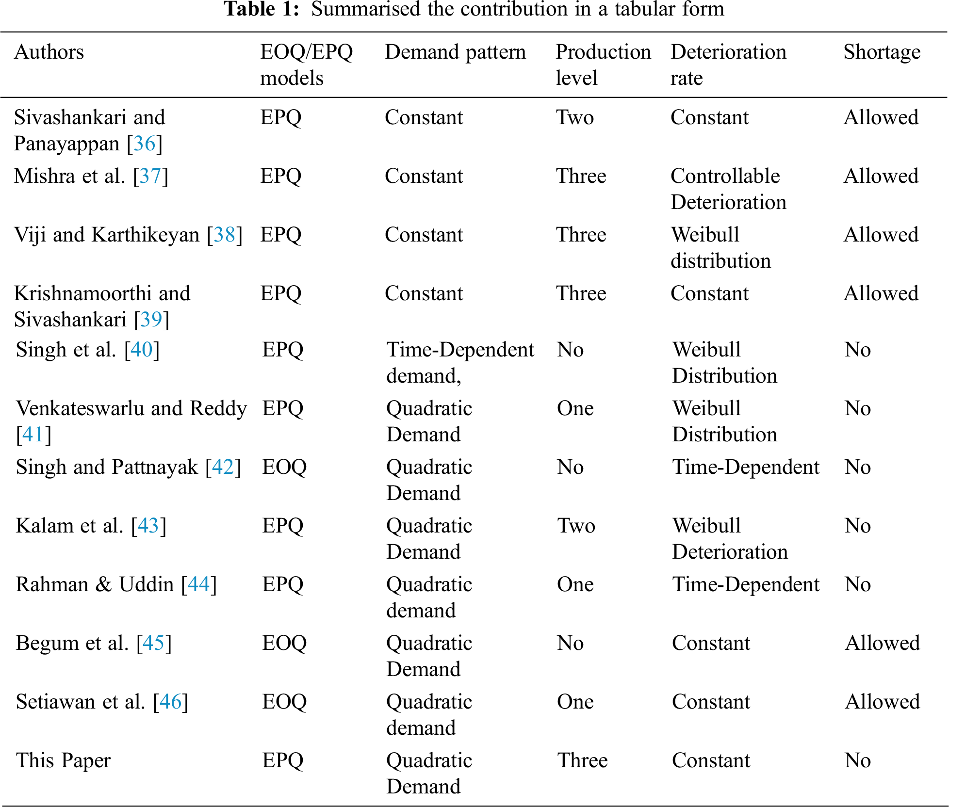
In a conventional inventory model, a steady demand rate is accepted. However, lately, numerous specialists have focused their consideration on a period subordinate demand approach. Acknowledging a steady demand rate is not always reasonable for some inventory things like trendy garments, electronic supplies, delicious food sources, etc. For this kind of model, the demanding work is subject to time. For instance, the radio has considered numerous individuals over twenty years prior, yet it is almost antedated these days. To mirror the circumstance in all the more obvious ways. The exertion of researchers who used constant, linear, and quadratic demand with one, two, and three production levels whereas with and without shortage models summarized in Tab. 1.

Nowadays, different types of demand are measured, such as linear demand, constant demand, quadratic demand, etc. Most scholars have work on continuous and linear trend demand, but few scholars work on quadratic requests. Singh [47] has fostered a solitary purchaser, single provider stock model with stock and time quadratic ward interest for a limited arranging distance has been contemplated. Single breaking down thing which smarts deficiency, with halfway accumulating and some lost deals thought. Kumar and Inaniyan [48] present a model that fosters a renewal strategy where the interest rate is quadratic polynomial-time work. The crumbling rate is a Pareto-type work. Deficiencies are fractional multiplying, and postponement in installments is permitted. Holding cost is a straight capacity of time. Patro et al. [49] have fostered a fluffy stock framework for time subordinate quadratic interest rate with Weibull deterioration rate, and the shortage is allowed partially backlogged. It is seen that an immense heap of things showed in a hypermarket will spur the client support to purchase more items. Along these lines, the participation of stock has an inspirational result on individuals around it. Also, there may be sporadic shortages in inventory due to many explanations.

1.3 Research Gap and Contribution

Sivashankari and Panayappan [36] analyzed the production stock model with deteriorative things in which two unique paces of productions are conceivable that production began at one rate. After some time, it very well might be exchanged another rate such a circumstance is alluring as starting at a low pace of production. Some authors explained that three unprecedented production levels and the deficiencies are allowed and ultimately delay purchased are described by Mishra et al. [37], Viji and Karthikeyan [38], Krishnamoorthi, and Sivashankari [39]. Singh et al. [40] proposed a decaying thing that follows three-boundary Weibull dissemination crumbling. Deficiencies are not allowed in this model. Venkateswarlu and Reddy [41], Singh and Pattnayak [42], Kalam et al. [43], and Rahman and Uddin [44] described production size stock models for disintegrating things with time subordinate quadratic interest rate. It expects that the disintegration rate follows time-dependent, Weibull circulation. The holding cost is a constant and straight capacity of time. Stock models create without thinking about deficiencies. Begum et al. [45] and Setiawan et al. [46] manages a stock model for weakening things alongside time subordinate interest which is the quadratic capacity of time. A mathematical model was created considering Weibull weakening for unique demand and quadratic demand with deficiencies of time-subordinate merchandise. The outcomes and affectability examination led and tracked down that inventory’s total expense will increase as per the demand and weakening of merchandise. No one considered the point (i) EPQ (ii) quadratic demand (iii) three-level production and (iv) deterioration rate derived the inventory model.

The suppositions and notations of the model are begun in segment 2. Then, the numerical model is inferred in area 3; the arrangement method and calculation determine in segment 4, and numerical delineation and sensitivity investigation are discussed in segment 5. The managerial insights and practical implications are explained in section 6. Finally, at the finishes for specific conclusion comments and the extent of future research scope in segment 7.

2  Suppositions and Notation

2.1 Suppositions

The suppositions of an inventory model are as follows:

1.    The production amount is known and constant.

2.    The requested rate is the straight capacity of time and is nonnegative.

3.    Three rates of manufacture are considered.

4.    The item is a sole product; it does not subordinate with additional inventory substances.

5.    The production rate is consistently grandiose or equivalent to the amount of the interest rate.

6.    The principal time is assuming zero.

7.    The replenishment rate is finite.

2.2 Notation

(a)   p – Production amount in the unit of time.

(b)   D – Demand rate in units per unit time, where D = (a + bt + ct2) and a,b & c>0 .

(c)   θ – Deterioration rate is constant.

(d)   R1 – Inventory close at time T1.

(e)   R2 – Inventory close at time T2.

(f)   R3 – Inventory near at the time T3.

(g)   cp – Production cost per unit.

(h)   cd – Deterioration cost.

(i)   hc – Holding cost per unit time.

(j)   k – Setup cost per production cycle.

(k)   T4 – The Length of the inventory cycle.

(l)   Ti – Unit time in periods, i=1,2 & 3 .

3  Mathematical Model and Solution

Each rotation begins with the primary opening business sector and stops with the last shutting market. The demand rate is time-subordinate. Allow us to accept that the production started at the time down t = 0 and finished on time t = T4. Throughout the time interlude, [0, T1] let the production rate p and demand rates (a + bt + ct2) where a,b & c are positive value and D is less than p. The stock accomplishes a level R1 at a time t = T1, amid the time interims [T1, T2] and [T2, T3] the mounting rate to be measured as d(p − D) and e(p − D) where d and e are constants. The relation between d and e are (e > d > 1). The inventory level achieves R2 and R3 at the times T2 and T3 respectively. At the time T3, production stopped after that inventory level reduced due to the combined effect of demand and deterioration. Inventory level reduces to zero levels at a time T4. The geometry of the model has been show in Fig. 1.

Let Q(t) be the inventory level at time t. The differential conditions portraying the framework in the stretch (0, T4) are given by

dQ(t)dt+θQ(t)=p−(a+bt+ct2);0≤t≤T1 (1)

dQ(t)dt+θQ(t)=d{p−(a+bt+ct2)};T1≤t≤T2 (2)

dQ(t)dt+θQ(t)=e{p−(a+bt+ct2)};T2≤t≤T3 (3)

dQ(t)dt+θQ(t)=−(a+bt+ct2);T3≤t≤T4 (4)

With boundary conditions

Q(0)=0, Q(T1)=R1, Q(T2)=R2, Q(T3)=R3& Q(T4)=0 (5)

Solution of the differential Eqs. (1)–(4) using boundary conditions (5) are as follow:

Q(t)= (2ce−tθ−2c−bθe−tθ+bθ+2ctθ+aθ2e−tθ−aθ2−Pθ2e−tθ+Pθ2−btθ2−t2θ2)θ3,0≤t≤T1 (6)

Q(t)= d(2ce−tθ−2c−bθe−tθ+bθ+2ctθ+aθ2e−tθ−aθ2−Pθ2e−tθ+Pθ2−btθ2−t2θ2)θ3,T1<t≤T2 (7)

Q(t)= e(2ce−tθ−2c−bθe−tθ+bθ+2ctθ+aθ2e−tθ−aθ2−Pθ2e−tθ+Pθ2−btθ2−t2θ2)θ3,T2<t≤T3 (8)

Q(T)= −1θ3[e−tθ(2cetθ−2ceTθ−betθθ+beTθθ−2cetθtθ+2ceTθTθ+aetθθ2−aeTθθ2+betθtθ2+cetθt2θ2−beTθTθ2−ceTθT2θ2)],T3<t≤T4 (9)

Maximum inventory level R1: The maximum inventory level during the period (0, T1) is solved as follows from the Eqs. (5)–(6), Q(T1)=R1

Growing the exponential term and neglecting the third term and higher power of theta for small value of theta, we get

R1=θ3T12[bT1+2a−aT1θ−2P+PθT1] (10)

Maximum inventory R2: The supreme stock level throughout the period (T1, T2) is solved as follows from the Eqs. (5)–(7), Q(T2)=R2

Escalating the exponential term and overlooking the third term and higher power of theta for the minor value of theta, we get

R2=dT2θ32[bT2+2a−aT2θ−2P+PθT2] (11)

Maximum inventory R3: The maximum inventory level during the period (T2, T3) is solved as follows from Eqs (5)–(8), Q(T3)=R3

Expanding the exponential term and neglecting the third term and higher power of θ for the small value of θ, we get

R3=eT3θ32[bT3+2a−aT3θ−2P+PθT3] (12)

4  Cost Calculation of Proposed Inventory Model

1. Production cost PC = D cp (13)

2. Set up cost TSc = K (14)

3. Holding cost of per unit time THc

Escalating the exponential functions and ignoring second and higher power ofθ, whereasθ is very small then equation reduces to a new form.

=hc[1θ4{a−p−T12θ33+(p−a)θ2+(p−a)T12θ42}+16θ4d(T1+T2)(6cT1θ2−6cT2θ2)+d(T1−T2)T1T2θ2(3bT1θ2+3bT2θ2+2T12θ2+2T22θ2+2T1T2θ)+6d(T1−T2)=+(bθ3T1+aθ4T1−pθ2T1)+16θ4d(T2+T3)(6cT2θ2−6cT3θ2)+d(T2−T3)T2T3θ2=(3bθ2(T2+T3)+2θ2(T22+2T32)+2T2T3θ)+6d(T2−T3)(bθ3T2+aθ4T2−pθ2T2)+16θ4T33θ2(3b−4c)+T42θ2(3b−6c)+4cT43θ3+θ2T2T4(12c−6bθ−6cT4)] (15)

4.1 Deterioration Cost of Finished Products

Mounting the exponential functions and overlooking second and higher power of θ then

=θcd[1θ4{a−p−T12θ33−aθ2−aT12θ42+pθ2+pT12θ42}+16θ4d(T1+T2)(6cT1θ2−6cT2θ2)+d(T1−T2)T1T2θ2(3bT1θ2+3bT2θ2+2T12θ2+2T22θ2+2T1T2θ)+6d(T1−T2)+(bθ3T1+aθ4T1−pθ2T1)+16θ4d(T2+T3)(6cT2θ2−6cT3θ2)+d(T2−T3)T2T3θ2(3bθ2(T2+T3)+2θ2(T22+2T32)+2T2T3θ)+6d(T2−T3)(bθ3T2+aθ4T2−pθ2T2)=+16θ4T33θ2(3b−4c)+T42θ2(3b−6c)+4cT43θ3+θ2T2T4(12c−6bθ−6cT4)] (16)

The all-out cost of the proposed stock model TC = PC + TSC + THc + TDc

TC=[K+cp(a+bT4δ)+(hc+cdθ)θ4[{a−p−T12θ33−aθ2−aT12θ42+pθ2+pT12θ42}+16θ4d(T1+T2)(6cT1θ2−6cT2θ2)+d(T1−T2)T1T2θ2(3bT1θ2+3bT2θ2+2T12θ2+2T22θ2+2T1T2θ)+6d(T1−T2)+(bθ3T1+aθ4T1−pθ2T1)+16θ4d(T2+T3)(6cT2θ2−6cT3θ2)+d(T2−T3)T2T3θ2(3bθ2(T2+T3)+2θ2(T22+2T32)+2T2T3θ)6d(T2−T3)(bθ3T2+aθ4T2−pθ2T2)+16θ4T33θ2(3b−4c)+T42θ2(3b−6c)+4cT43θ3+θ2T2T4(12c−6bθ−6cT4)] (17)

Let T1=αT4T2=βT4 & T3=γT4 therefore the total cost will be becoming

=[K+cp(a+bT4δ)+(θcd+hc)6θ46a−6aθ2+aT4(α−3T4α2+6eT4β(β−γ))θ4−6p+6pθ2+pθ2T4(6eT4β(−β+γ)−α+3T4α2θ2)+T4(d(α−β)(6+6cT4(α+β)θ2+T43αβθ3(3b(α+β)θ+2T4(αβ+α2θ+β2θ))+θ2(bαθ+3bT4(1+T4γ3−2(γ+eβ(γ−β))θ+eT42β(β2−γ2)γθ2+2T4(6cγ−3cγ−3cT4γ−2T4γ3+3ce(β2−γ2)+2cT4θ−θα2+eT43β(β−γ)γ(βγθ+β2θ2+2γ2θ2))))] (18)

Objective

The study’s objective is to investigate the optimal time T4∗ , which minimizes TC as follows and then differentiates with respect to T4.

dTCdT4=[bδcp+(θcd+hc)6θ46(b−2c)T4θ2+2d(α−β)(3+6cT4(α+β)θ2+T43αβθ3(6b(α+β)θ+5T4(αβ+(α2+β2)θ)))+θ2(9bT42γ3+24cγT4−18T42γ−12T42γ312ecT4(β2−γ2)bα+θ(12cT42+10eT44β2(β−γ)γ2−4T4(α2+3b(γ−eβ2+eβγ))+θ2(aα−6Ta4α2+12aeT4β(β−γ)+2eT43β(β−γ)γ(6b(β+γ)+5T4(β2+2γ2)))+12epT4β(−β+γ)−α+6T4pα2θ2))] (19)

Again, differentiate concerning T4 the equation will be

d2TCdT42=[(θcd+hc)3θ23b−6c+9bT4γ3−2α2θ−6bγθ−3aα2θ2+3pα2θ2+12cγ−18cT4γ−12cT4γ3+6ce(β2−γ2)+12cT4θ)d(α−β)(6c(α+β)+2T42αβθ(9b(α+β)θ+10T4(αβ+α2θ+β2θ)))+2eβ(β−γ)(−3p+3bθ+3aθ2+9bT42γ(β+γ)θ2+10T43γθ(βγ+β2θ+2γ2θ))] (20)

d2TCdT42>0 , Solving Mathematica software 9.0.

5  Numerical Analysis

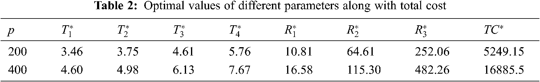
Example 1: The accompanying information has been considering to approve the proposed model. Creation rate is $200, the demand rate of parameter a=5,b=4,c=3,d=2.5 & e=3 unit, production cost is $10; deterioration cost $2, set-up cost $200, holding cost $0.2 per unit, α=0.6,β=0.7 & γ=0.8 deterioration rate is $0.2. The optimal value of T1∗,T2∗,T3∗ & T4∗ an entire inventory of R1∗,R2∗ & R3∗ and optimal total cost TC∗ has been intended with the support of Eqs. (19), (10–12), (17), shown in Tab. 2.

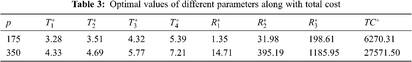
Example 2: The additional information has been considering to approve the proposed model. Production rate is $175, the demand rate of parameter a=5.2,b=4.2,c=3.2,d=2.6 & e=3.6 unit, production cost is $10; deterioration cost $2, set-up cost $200, holding cost $0.5 per unit, α=0.6,β=0.7 & γ=0.8 deterioration rate is $0.2. The optimal value of T1∗,T2∗,T3∗ & T4∗ an entire inventory of R1∗,R2∗ & R3∗ and optimal total cost TC∗ has been intended with the support of Eqs. (19), (10–12), (17), shown in Tab. 3.

5.1 Sensitivity Analysis

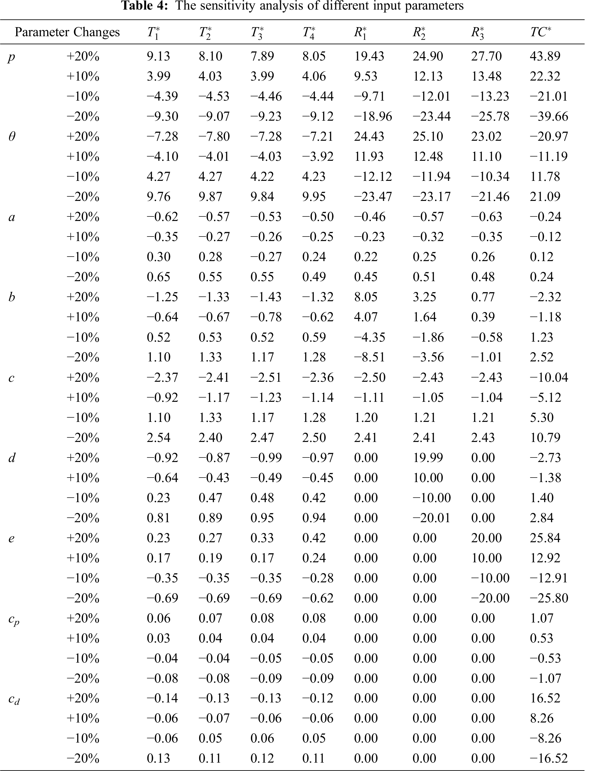
As an outcome of changes in the various parameters of the proposed model, the sensitivity investigation is proficient by thinking about 10% and 20% increment or decline in each of the above parameters, keeping the remaining parameter the equivalent. The affectability examination finished by changing the specified parameters p,θ,a,b,c,d,e,cp & cd by Tab. 4. This table shows the sensitiveness of the various parameters on the optimal values of T1∗,T2∗,T3∗,T4∗,R1∗,R2∗ & R3∗ , over-all cost TC∗ .

The optimal values of T1∗,T2∗,T3∗ & T4∗ slightly change with the values of the parameters a,b,d,e,cp & cd , moderately for b & d and highly with p & θ .

The optimal value of R1∗,R2∗ & R3∗ slightly change with the value of the parametera, moderately with b & c and highly with p,θ,d & e .

The optimal value of TC∗ slightly changes with the values of the parameters a,b,d & cp moderately changes with parameterc and highly with the values of p,θ,e & cd .

5.2 Graphical Analysis

The graphical illustration is a method of breaking down mathematical information. It shows the connection between data, thoughts, and ideas in a chart. It is straightforward, and it is quite possibly the principal learning methodologies. It generally relies upon the sort of data in a specific area. The graphical representation of the optimal total cost concerning the optimal time T4∗ that is the convexity of TC∗ concern T4∗ has been shown in Fig. 2. and Fig. 3. respectively as follow:

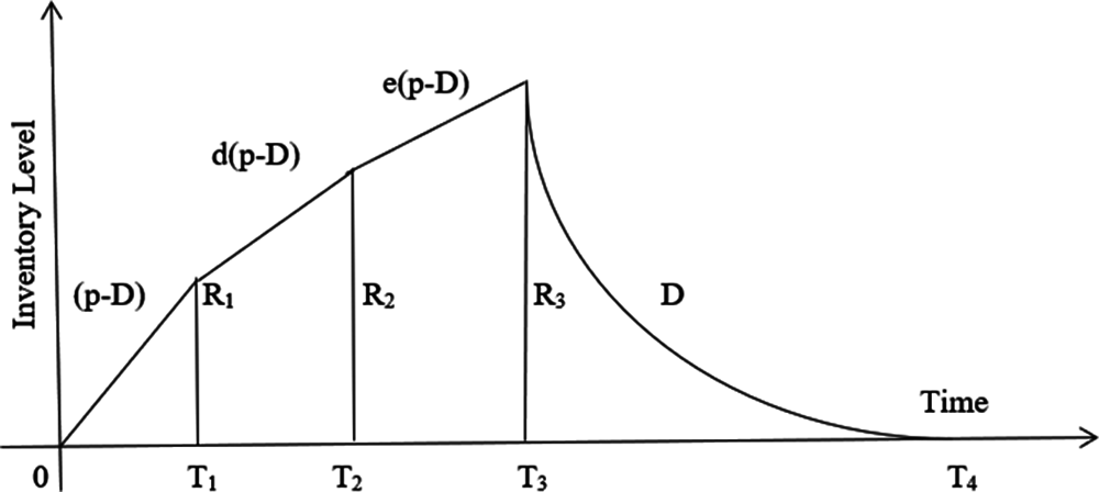
Figure 1: Geometry of the production inventory level without shortage

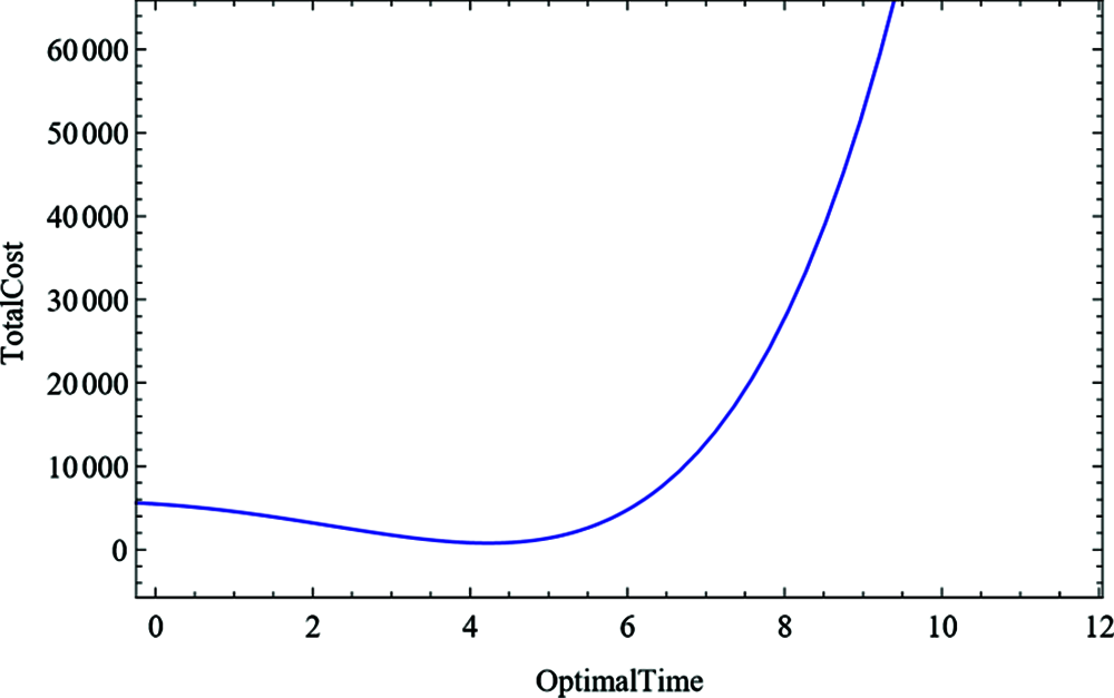
Figure 2: Optimal value of TC w.r.t T4∗ when p = 200

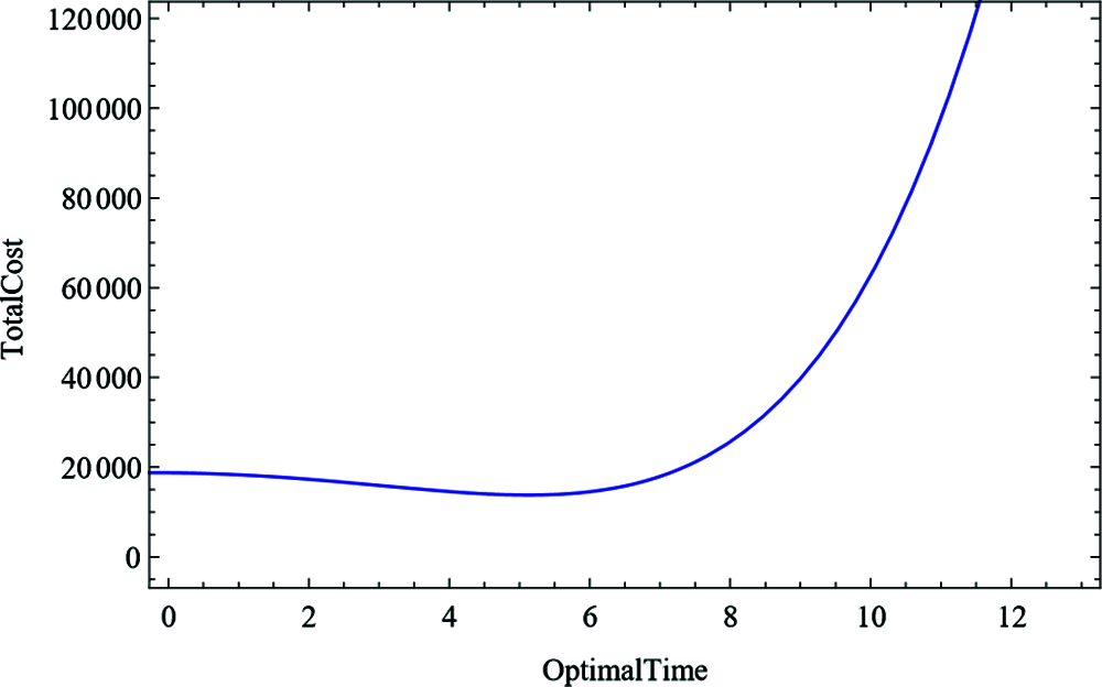
Figure 3: Optimal value of TC w.r.t T4∗ when p = 400

6  The Managerial Insights and Practical Implication

In this study, the developed structure can mimic real-world problems in three-phase quadratic demand where disturbance happens because of limit, order, catastrophic events, or unsure circumstances. Some commonsense ramifications of this examination are underneath: The quadratic demands administrators and professionals need to consider to handle the disturbance hazards related to dealing with a certain degree of inventory to guarantee reasonableness. Since our model, choices are profoundly affected by the irregular nature of the limit. It can lead the concerned staff to improve their inventory model.

Practical Implication of Model: This model controls exact non-prompt weakening things like electronic parts, food things, and trendy items. To diminish production cost and ultimately boost benefit, it is of most extreme significance to direct buy choices through some thorough inventory strategy, so production lines don’t run dry. Our model can lead them into dealing with the inventory framework in an advanced manner for this situation.

7  Conclusion

The planned model is exact for a dispatched item with a steady plan to a limited extent in time-subordinate interest. Because of this, we will get buyer fulfillment and procure more potential profit. The variety in production rate gives about customer fulfillment and making an expected benefit. A mathematical model provides to exhibit its reasonable utilization. Result approval is a significant advance in this examination. A circumstance is alluring as in by beginning at a low pace of production. An enormous quantum supply of assembling things at the underlying stage is kept away from, prompting a decrease in the holding cost. The variety in production rate gives way coming about shopper fulfillment and acquiring expected profit. A mathematical model and its affectability examination are provided. For validation, the model solves in Mathematica Software Basic 9.0. The anticipated stock model can help the producer and retailer to decide the ideal request amount, process duration, and final stock expense.

For further research: This model can be expanded in numerous ways involving diverse demand rates such as constant, quadratic, Weibull deterioration with three parameters, cubic demand, time discounting, and rework of defective items. We can also generalize the model in several ways: the time value of money, quantity discounts, price discounts, and rework of faulty items.

Acknowledgement: The author would like to thank the editor and anonymous reviewers for their valuable and constructive comments, which have led to a significant improvement in the manuscript. The first author is also thankful to IIT (ISM) Dhanbad for providing faculities.

Funding Statement: The authors received no specific funding for this study.

Conflicts of Interest: The authors declare that they have no conflicts of interest to report regarding the present study.

This work is licensed under a Creative Commons Attribution 4.0 International License, which permits unrestricted use, distribution, and reproduction in any medium, provided the original work is properly cited.