DOI:10.32604/iasc.2022.020178
| Intelligent Automation & Soft Computing DOI:10.32604/iasc.2022.020178 | |
| Article |
Breast Cancer Detection and Classification Using Deep CNN Techniques
1Department of CSE, National Engineering College, Kovilpatti, 628503, India
2Department of EEE, National Engineering College, Kovilpatti, 628503, India
*Corresponding Author: R. Rajakumari. Email: rajakumarinatarajan@gmail.com
Received: 12 May 2021; Accepted: 30 July 2021
Abstract: Breast cancer is a commonly diagnosed disease in women. Early detection, a personalized treatment approach, and better understanding are necessary for cancer patients to survive. In this work, a deep learning network and traditional convolution network were both employed with the Digital Database for Screening Mammography (DDSM) dataset. Breast cancer images were subjected to background removal followed by Wiener filtering and a contrast limited histogram equalization (CLAHE) filter for image restoration. Wavelet packet decomposition (WPD) using the Daubechies wavelet level 3 (db3) was employed to improve the smoothness of the images. For breast cancer recognition, these preprocessed images were first fed to deep convolution neural networks, namely GoogleNet and AlexNet for Adam. Root mean square propagation (RMSprop) and stochastic gradient descent with momentum (SGDM) optimizers were used for different learning rates, such as 0.01, 0.001, and 0.0001. As medical imaging necessitates the presence of discriminative features for classification, the pretrained GoogleNet architectures extract the complicated features from the image and increase the recognition rate. In the latter part of this study, particle swarm optimization-based multi-layer perceptron (PSO-MLP) and ant colony optimization-based multi-layer perceptron (ACO-MLP) were employed for breast cancer recognition using statistical features, such as skewness, kurtosis, variance, entropy, contrast, correlation, energy, homogeneity, and mean, which were extracted from the preprocessed image. The performance of GoogleNet was compared with AlexNet, PSO-MLP, and ACO-MLP in terms of accuracy, loss rate, and runtime and was found to achieve an accuracy of 99% with a lower loss rate of 0.1547 and the lowest run time of 4.14 minutes.
Keywords: Deep learning; breast cancer; DCNN; GoogleNet; AlexNet; PSO; MLP; image classification
Breast cancer is a commonly occurring cancer type, especially in women, compared to other types like lung and bronchus, colon and rectum, and uterine corpus [1,2]. Even with numerous advancements in diagnosis and treatment methods, a large number of annual mortalities occur [2]. Long-term mortality mainly results from the size of the tumor [3], making the detection of breast cancer less than two cm essential [4]. Identifying and treating breast cancer at an early stage is needed to reduce the death rate [5]. Mammography, which uses low-energy electromagnetic waves, is used for breast cancer imaging and is considered the most efficient method for detection at an incipient stage. Therefore, an accurate computer-aided classifier is required to reduce the risk of a wrong verdict due to asthenopia, lethargy, or a lack of skillset.
In the past years, several breast cancer recognition methods have been developed, and the performance of computer-aided recognition has been verified for a dataset taken from the UCI machine-learning repository. The breast cancer recognition rates of the optimized learning vector quantization (LVQ) method, bigLVQ method, and artificial immune system were 96.7%, 96.8%, and 97.2%, respectively [6]. The classification rate was found to attain 94.74% accuracy for the decision tree method with C4.5 using a 10-fold cross [7]. The fuzzy clustering method using supervisory control yielded a 95.57% accuracy rate, and a neuro-fuzzy classifier achieved 95.06% [8]. The breast cancer classification accuracy of the Wisconsin Breast Cancer (WBC) dataset by three classifiers, namely multi-layer perceptron (MLP), naïve Bayes (NB), and decision tree, was compared. A fusion classifier made of the MLP and J48 classifier was found to be superior [9]. A 96% recognition rate was achieved for breast cancer classification with RIAC [10], and around 98.53% was achieved with least square support vector machines (LSSVM) [11]. The performances were compared in terms of accuracy sensitivity specificity, and the high accuracy rate of LSSVM was determined to be due to its robustness nature. The feature reduction-based breast cancer decision system was explored via independent component analysis. The substantiated single dimension feature was sufficient to increase the radial basis neural network accuracy up to 90.49 [12]. Breast cancer images possess textural information that could bear discriminant features. Accordingly, the Laws’ texture features were extracted from mammograms to differentiate the normal and abnormal pixels. A wavelet network based on particle swarm optimization (PSO) was employed to detect breast cancer abnormalities using texture energy measured from mammograms, and it achieved 93.671%, 92.105%, and 94.167% accuracy, specificity, and sensitivity, respectively [13]. Detection of breast cancer using a deep belief network unsupervised path with Liebenberg Marquardt learning produced an accuracy of 99.68% for the WBC dataset [14].
A knowledge-based system using fuzzy logic was applied for breast cancer recognition by employing maximization for clustering the data. The problem of multi collinearity was avoided using principal component analysis [15]. An extreme learning machine classifier classified the benign and malignant breast masses using fused deep features, morphological features, texture features, and density features and achieved an 86.50% recognition rate. Even though many algorithms and techniques have developed for the classification of breast cancer images, further research is required to achieve greater accuracy in saving human lives. For this purpose, the following methods are proposed in this work: First, the Digital Database for Screening Mammography (DDSM) dataset images used for this research are discussed; these images were subjected to noise removal and image restoration using the Wiener filter, a contrast limited histogram equalization (CLAHE) filter, and wavelet tree decomposition before being subjected to feature segmentation. The reconstructed images were then fed to a deep convolutional neural network (DCNN)-based GoogleNet model, which has an inception approach for feature extraction at the training and testing phase. The performance of GoogleNet was compared with AlexNet. The programming environment used for the implementation of this proposed work was MATLAB 2019. Second, the statistical features of the images, such as skewness, kurtosis, variance, entropy, contrast, correlation, energy, homogeneity, and mean, were extracted from the preprocessed images and fed as the input to a particle swarm optimization-based multi-layer perceptron (PSO-MLP) and an ant colony optimization-based multi-layer perceptron (ACO-MLP) for breast cancer recognition.
This paper is structured as follows: Section 2 explains the preprocessing of breast cancer images using the Wiener filter, the CLAHE filter, and wavelet packet decomposition. Section 3 covers the proposed methodology, classifiers, and initialization parameters. Finally, Section 4 discusses the results and comparison of different classifiers, and Section 5 concludes with the impact of this work
2 Preprocessing of Breast Cancer Images
Images were taken from the DDSM for breast cancer recognition work. This database contains normal, malignant, and benign cancer images with 650 pictures for each category. The DDSM images were preprocessed to remove background noise and augment the contrast between the cancer cells and the neighboring areas, which aids in localizing the region of interest (ROI). Feature extraction, training, and testing images were fed to the DCNN-based GoogleNet classifier.
2.1 Preprocessing of DDSM Images
Many preprocessing methods have been reported in Refs. [16–18]. The preprocessing approach adopted in this work is shown in Fig. 1.

Figure 1: Block diagram of breast cancer image preprocessing
The original DDSM images were converted into binary images, as shown in Fig. 2(b). Then, to increase the intensity of the breast and muscle elements and suppress the other, unwanted information, the binary image was multiplied using the original breast image given in Fig. 2(c). This process was carried out by increasing and decreasing the luminosity.

Figure 2: Preprocessing of breast cancer image for breast and muscle identification: (a) original image; (b) binary image; (c) identification of breast and muscles
The background was deleted in the image, as shown in Fig. 3(a), by deleting the zero-intensity pixels of the rows and columns. Gray thresholding based on Otsu’s method was applied to the processed image, and the intensity of the image was varied to a midpoint between the minimum and maximum levels of the original intensity; resultant muscle-removed image is shown in Fig. 3(b). Then, the breast image was fed to the Wiener filter to eliminate noise. Once the spectral power was estimated, a mask was applied to all the pixels of the original image with a signal-to-noise ratio (SNR) of 0.2. By using the mean and variance of the authentic images, a new mean, variance, and power were calculated for all the pixels of the transformed images.
2.2 Wiener and CLAHE Filtering
The Wiener filter’s characteristics offer a trade-off between inverse filtering and smoothening of noise; thus, it has the capability of simultaneously removing additive noise and blur inversion. Furthermore, the stochastic nature of the Wiener filter linearly estimates the normalized image based on the orthogonality expressed in Eq. (1).
where
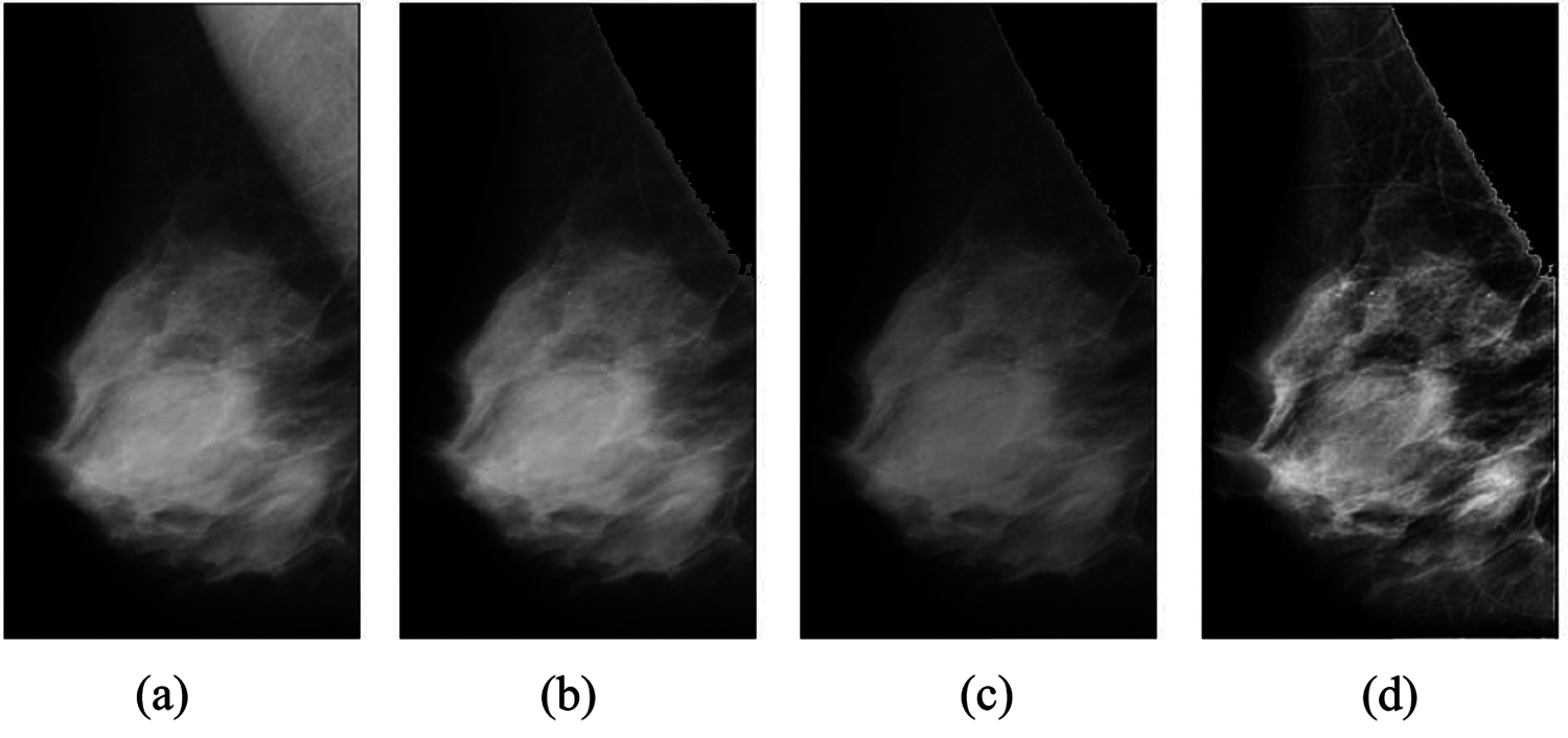
Figure 3: Breast cancer image before and after preprocessing: (a) background removed image; (b) muscle removed and breast alone present; (c) Wiener filter applied to image; (d) image after applying CLAHE filter
2.3 Wavelet Packet Decomposition (WPD)
Non-stationary and high-frequency noises were eliminated using wavelet packet decomposition. This method involves the use of windows of different lengths and is efficient in image denoising while preserving the edges and texture. In two-dimensional (2D) WPD, the breast cancer DDSM image is decomposed into sub-images containing details about the edges in horizontal, perpendicular, and transverse orientations. The 2D WPD generates one approximation coefficient and one detail coefficient in the horizontal, vertical, and diagonal orientations, with a total of four components for each level.
Eq. (2) provides the 2D WPD applied to the I(m, n), representing the breast cancer image of size m × n.
Eqs. (3)–(6) were used to generate the coefficients for the sub-band, with one low-frequency coefficient in both the horizontal and perpendicular regions (L–H, L–H) and three high-frequency coefficients, specifically, low frequency in the horizontal and high frequency in the perpendicular region (L–H, H–P), high frequency in the horizontal and low frequency in the perpendicular region (H–H, L–P) and high frequency in both the horizontal and perpendicular regions, which is the transverse orientation (H–H, H–P). Fig. 4 represents the wavelet packet decomposition of the image and its hierarchy for level 2.
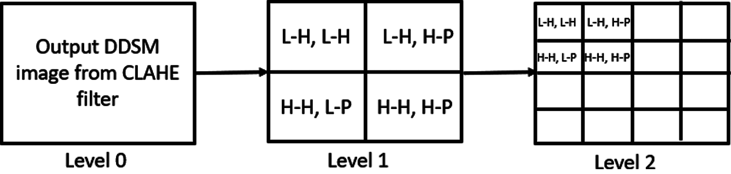
Figure 4: Wavelet packet decomposition of image for level 2
In this work, WPD using the Daubechies wavelet3 (db3) level 2 was employed, and the wavelet tree and reconstructed output image are shown in Fig. 5. The optimal tree was chosen by finding the cost function at each node using the Shannon entropy function: For any sub-band, if each parent’s cost function is greater than the cumulative sum of all the children nodes, the parent and child nodes are both retained; else, only the parent node is retained. This process is repeated up to level 2 of decomposition, which results in the quaternary tree. In the quaternary tree, each node represents the image in WPD. Node (0, 0) is the original image, and nodes (1, 0), (1, 1), (1, 2), and (1, 3) are the images obtained after level 1 decomposition. These, along with nodes (2, 0), (2, 1), (2, 2), (2, 3), (2, 4), (2, 5), (2, 6), (2, 7) up to (2, 15) and level 2 decomposition images, are shown in Figs. 5(a) and 5(b). Figs. 5(c) and 5(d) depict the WPD image and wavelet packet coefficients.
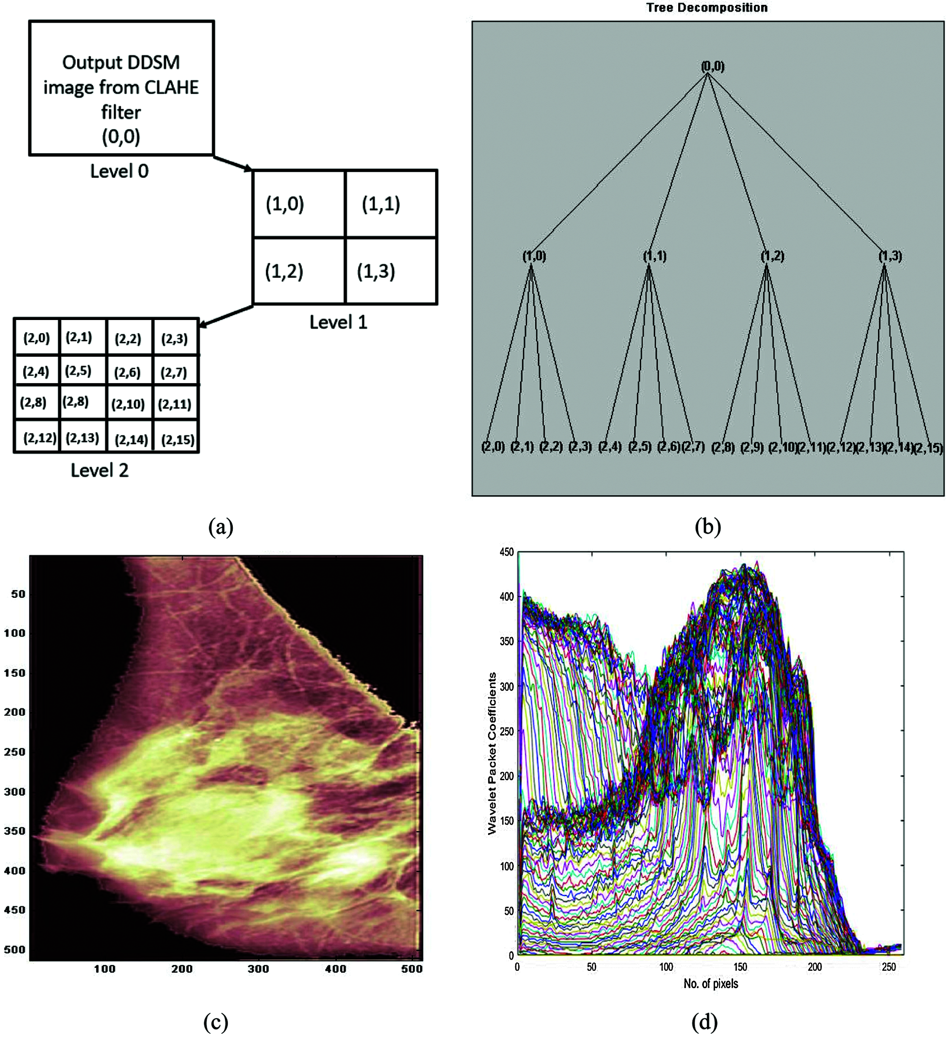
Figure 5: Breast cancer image decomposition using wavelet packets with db3: (a) image after applying CLAHE filter; (b) quaternary tree; (c) reconstructed breast cancer image after denoising using WPD; (d) wavelet packet coefficients
The database images were preprocessed and fed to the classifiers for breast cancer recognition. The images were resized to 224∗224 for GoogleNet and 227∗227 for AlexNet architecture. Subsequently, features such as skewness, kurtosis, variance, entropy, contrast, correlation, energy, homogeneity, and mean were extracted from the preprocessed images and fed as the inputs to PSO-MLP and ACO-MLP for cancer recognition. The flow of the proposed approach for the image-based recognition of breast cancer is depicted in Fig. 6.
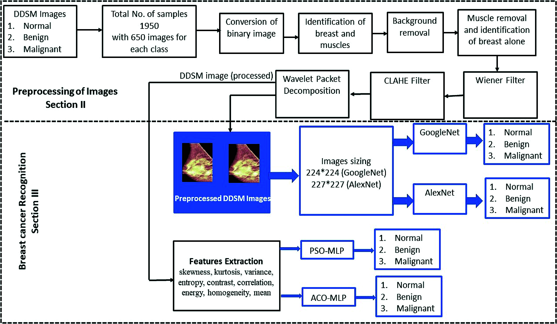
Figure 6: Proposed approach for breast cancer recognition
The pretrained deep learning convolution neural networks GoogleNet and AlexNet were considered for this work. For both these networks, images were resized and fed as inputs. Training and testing were done for a 70:30 proportion of the preprocessed images in both networks.
The GoogleNet model proposed in Szegedy et al. [19] is complex and goes deeper than all other CNN architectures. It has a 22-layer DCNN with an inception module, cascading various dimensions and sizes into a single new filter, as shown in Fig. 7.
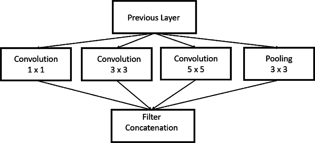
Figure 7: GoogleNet inception model
GoogleNet has a multiple features extractor in a single layer, which aids the network’s performance by choosing either to convolute the input or pool the information directly during training and image classification; the piling of this inception layer results in the final architecture. Each layer acts as a filter: the common features are detected in the starting layers, and the discriminating features are identified in the final layers. The inception layer covers a large area and retains a delicate resolution even for small information in an image. This property is maintained by convolving in a parallel approach with different sizes ranging from 1 × 1 to 5 × 5. Inception layers are employed with Gabor filters in series with various sizes having the learning capability. The convolution and pooling layers target the image features that are not necessary for training, thus reducing feature dimension and storage space. To avoid over fitting, nine inception modules are used in GoogleNet. The top layer consists of an output layer and both joint and parallel training, and this subtlety helps in faster convergence.
In this work, GoogleNet, which has a total of 144 layers, was retrained to classify breast cancer images by inserting four new layers into its structure: a dropout layer with a 50% probability of dropout, a fully connected layer, a softmax layer, and a classification–output layer with three outputs.
AlexNet is also a pretrained network [20] that has 11 × 11, 5 × 5, 3 × 3, convolution, max pooling, dropout, and fully connected layers with ReLU activation functions after every convolutional and fully connected layer. The dropout layer has a 50% probability of dropout. The fully connected layers are modified to three as there are three output classes.
DCNN networks are trained using the stochastic gradient descent with momentum (SGDM) optimization algorithm, root mean square propagation (RMSprop) optimizer, and adaptive momentum (Adam) optimizer along with transfer learning, which does not require many databases for achieving high accuracy. Optimizers are used to change the attributes of the neural network, such as weights and learning rate, to reduce losses. An optimizer is an algorithm used to update the various network parameters, and it can reduce the loss with little effort.
The learning rate is used to control the weight updation based on the error value. A low learning rate may result in a long time for training may get stuck, whereas a high value may yield a nominal weight value and result in instability. In training optimization, SGDM, Adam, and RMS prop update their descent algorithm weights based on the loss function value of each iteration.
Stochastic Gradient Descent with Momentum (SGDM) Optimization
The SGDM optimizer swings towards optimum through steepest descent path. The magnitude of swing can be limited by momentum [21]. Eq. (7) represents the weight updation process via SGDM optimization.
Here,
Root Mean Square Propagation (RMSprop) Optimization
RMSprop overcomes the drawback of the SGDM optimizer, as the same learning rate is used for all parameters. However, RMSprop implements various learning rates for the different parameters. Weight updation is done using Eq. (9), which is normalized by Eq. (8) based on loss function optimization [22].
where
Adaptive Momentum (Adam) Optimization
Adam also follows the RMSprop for weight updation method using momentum. Eqs. (10) and (11) are used to find the gradient parameter and the squared gradient parameter.
If the gradient remains constant for many iterations, then the pick-up momentum is used for the gradient’s moving average.
3.1.4 Training of GoogleNet and AlexNet
The present study was executed using the DDSM dataset with 1950 breast cancer images in total and 650 images for each of three classes: normal, benign, and malignant. The preprocessed image sizes were modified to 224∗224 and 227∗227, respectively, and fed to the pretrained GoogleNet and AlexNet.
The DDSM images were randomly divided for training and testing in a ratio of 70:30. In the training phase, the minimum batch size used was 20 images for each iteration. In this work, Mini Batch Size, Max Epochs, number of iterations, and Initial Learn Rate values were assigned as 10, 10, 100, and 0.0001, respectively. Ane poch refers to applying the training algorithm for all the training images. The training was done for three learning rates—0.01, 0.001, and 0.0001—with SGDM, Adam, and RMSprop as the optimizers. The simulations are carried out in MATLAB 2020b in an Intel Core Processor i7-7500U CPU at 2.70 GHz, 2904 MHz, two cores, and 64 GB of RAM.
A multilayer perceptron (MLP) is a feed-forward artificial neural network (ANN). MLP used nonlinear activation for all nodes except the input node and implements back propagation learning during training with the capability to distinguish nonlinearly separable data. The optimization process in MLP training involves finding the weights to minimize the mean square error. However, the back propagation algorithms based on the gradient descent method get locked in local minima as this algorithm efficiency depends on initial weights and bias values, and numerous iterations are required to tune the learning rate. To obtain the optimal weights of MLP networks, evolutionary-based approaches such as particle swarm optimization (PSO) [23] and Ant colony algorithm [24] are implemented, as fewer parameters require adjustment for better convergence.
3.2.1 Particle Swarm Optimization (PSO)-Based Multilayer Perceptron
The PSO algorithm is an outcome of birds’ flocking behavior and flying patterns, proposed by Kennedy and Eberhart in 1995. Each particle of PSO is characterized by position and velocity. In PSO, swarm particle size is represented by m’ and current instant by t; then, each particle between
mw is the inertia momentum is a scalar quantity used to control the degree of exploration in searching.
3.2.2 Ant Colony Optimization (ACO)-Based Multilayer Perceptron
The ACO algorithm is an outcome of the ant foraging behavior of finding the optimum path between the food source and destination. ACO can resolve a complex optimization problem when combined with another method. Based on the transition probability and pheromone quantity in that region, the pheromone trajectory is updated. The fitness value is calculated for the global ants produced in each iteration. If fitness improves upon updating the pheromone, then the local ant is moved to the better region, else the search is directed towards a new direction. ACO continues its local and global search by updating the pheromone and evaporating it. Eq. (16) expresses the transition probability in the region r, which is the measure of the local ant’s capability to move in a concealed region.
Here, L is the cost function for
3.2.3 Features Extraction and Training of PSO-MLP and ACO-MLP
Statistical features such as mean, skewness, kurtosis, variance, entropy, contrast, correlation, energy, and homogeneity were extracted from the preprocessed images and fed as inputs to the PSO-MLP and ACO-MLP for breast cancer recognition.
Mean indicates the brightness of the image and is calculated using Eq. (19).
where ∑∑ p(i,j) is the summation of pixel values, and (m∗n) is the image size.
Skewness reflects the disproportionate pixel value distribution used to measure the dark lustrous portion and is calculated using Eq. (20). The standard deviation is calculated using Eq. (20a).
Kurtosis measures the tendency of the peak with normal distribution, which is calculated using Eq. (21).
Variance is a measure of the contrast of the image and is calculated using Eq. (22).
Entropy determines the randomness nature and texture characterization, and it is calculated using Eq. (23).
Contrast represents the difference between an image’s maximum and minimum pixel intensity values and is calculated using Eq. (24).
Correlationis obtained in the following way. Filter mask is moved over the image, and the sum of products is evaluated in each region and used to detect the object in the image, irrespective of its position in the image, using Eq. (25).
where
Energy measures the gray level distribution, and it is based on an image normalized histogram; it is calculated using Eq. (26).
Homogeneity describes how values of a pixel vary in the image, and it is calculated using Eq. (27).
The structure used for PSO-MLP and ACO-MLP for breast cancer images is shown in Fig. 8, and the parameters used are listed in Tab. 1.

Figure 8: PSO/ACO-MLP structure

4 Experimental Results and Discussion
GoogleNet, AlexNet, PSO-MLP, and ACO-MLP classifiers were trained to categorize the DDSM breast cancer images into three categories based on their extracted features and corresponding labels: normal, benign and malignant. The test images, which fall under the diagnosis breast cancer images, were classified using this trained network. Soft tissue images are sometimes hard to see using other imaging tests. However, our proposed detection approach is very good at finding and pinpointing some cancers. An MRI with contrast dye is the best way to visualize brain and spinal cord tumors. Using processed images, the present study’s approach can physically interpret if a tumor is cancer.
4.1 Recognition Using GoogleNet and AlexNet
Figs. 9 and 10 show the performance accuracy and loss function value of GoogleNet and AlexNet, respectively, with a learning rate of 0.001. The graphs are presented for a single epoch only for better visualization. The performance of both GoogleNet and AlexNet classifiers varies with learning rate, and the highest accuracy is achieved with a low learning rate. It is evident from Fig. 8 that GoogleNet achieves 98.23% accuracy in the first epoch with the Adam optimizer and becomes oscillatory. It becomes stable until the maximum iteration for a low learning rate of 0.001, and it is clear that the loss function is greatly reduced and remains constant after the 50th iteration. As Fig. 9 shows, 96.19% accuracy is achieved by AlexNet only with the Adam optimizer. Both GoogleNet and AlexNet have low loss function valuations around the 50th iteration and remain stable with the Adam optimizer. Neither GoogleNet nor AlexNet shows a stable learning process for a high learning rate.
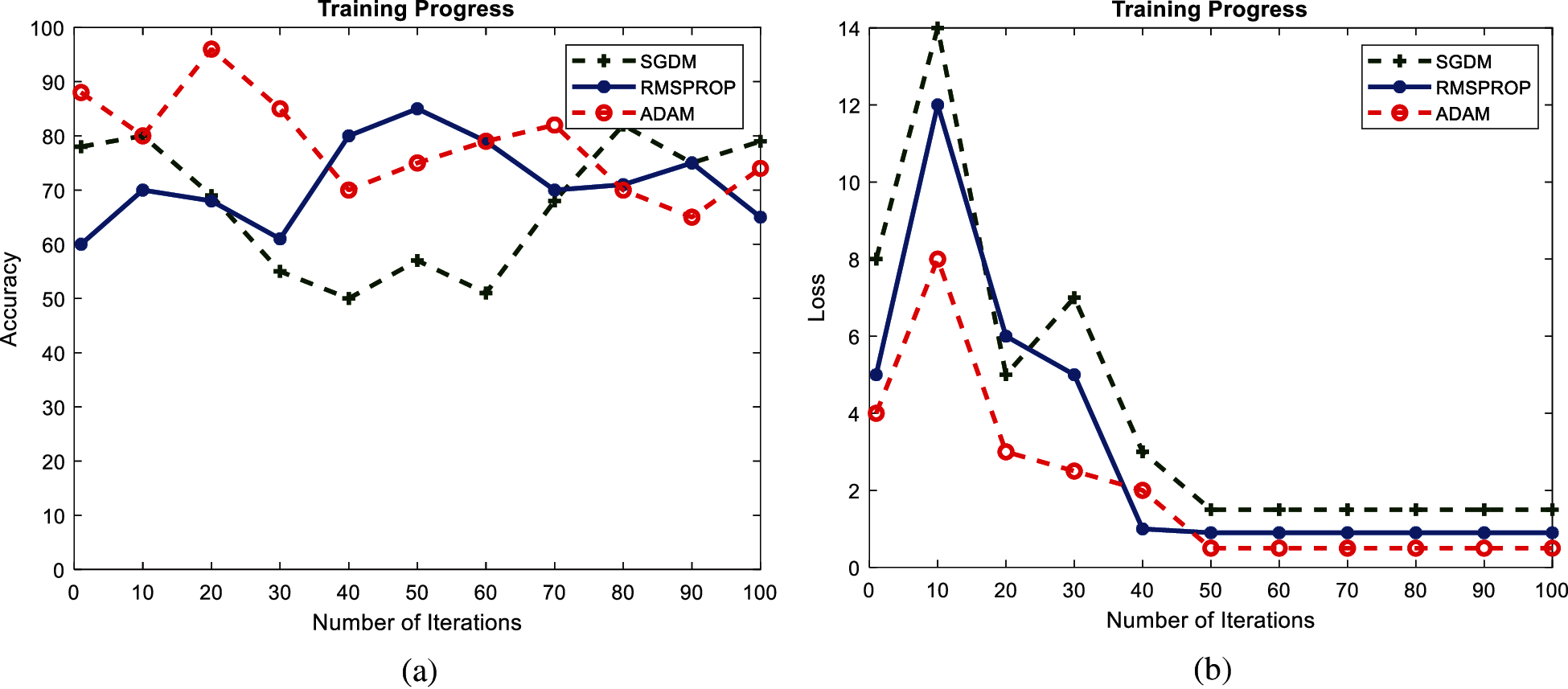
Figure 9: Performance curves of GoogleNet during training with learning rate 0.001: (a) accuracy; (b) loss function
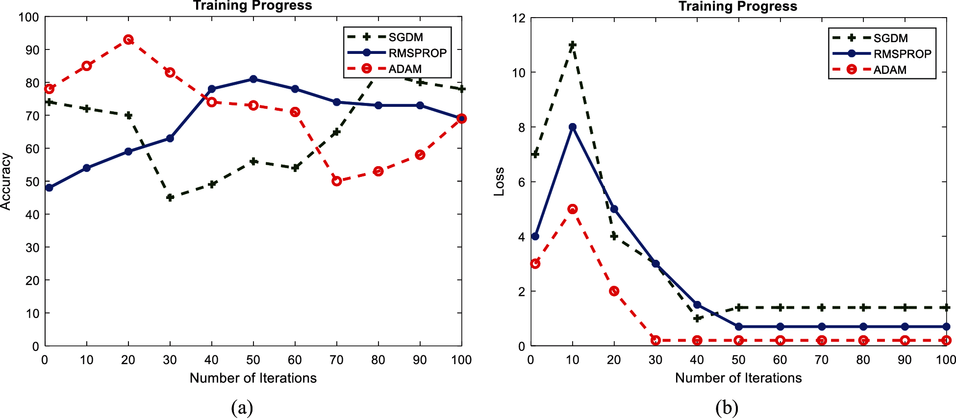
Figure 10: Performance curves of AlexNet during training with learning rate 0.001: (a) accuracy; (b) loss function
Tabs. 2 and 3 showcase the performance of GoogleNet and AlexNet, respectively, in classifying DDSM images for breast cancer. It is clear that network performance increases with a decrease in the learning rate in both networks.


During training, the maximum accuracy recorded was 98.23% for GoogleNet. In contrast, 97.97% was the recognition accuracy for the GoogleNet and AlexNet’s test data training with Adam as optimizer and learning rate as 0.001. During testing, GoogleNet yielded an accuracy of 99% with a learning rate of 0.001 and the Adam optimizer. Still, the accuracy achieved by AlexNet was 98.91% for a learning rate of 0.001 with the RMSprop optimizer; this was slightly higher than the 98.80% accuracy for Adam with the same learning rate. The performance was also measured in terms of runtime during the process: The lowest run time measured was 4.14 minutes with a 0.001 learning rate for Adam, and the highest run time recorded was 5.56 for SGDM with a 0.01 learning rate in GoogleNet. For AlexNet, the lowest run time was 4.71 minutes with the Adam optimizer and a 0.001 learning rate and the highest run time was 5.91 minutes with SGDM and a 0.01 learning rate. Both the networks show superior performance with a low learning rate of 0.001 and the Adam optimizer. In comparison, GoogleNet outperforms AlexNet in terms of accuracy and runtime and shows exemplary image processing performance for detecting breast cancer. Further, in existing works, the extreme learning machine classifier has achieved 86.5% and PSO-MLP has achieved 90.21% for the statistical features.
4.2 Comparison of Breast Cancer Recognition of GoogleNet with PSO/ACO-MLP
PSO-MLP and ACO-MLP classifiers were trained and tested in the proportion of 70:30 of preprocessed images. The recognition rates of PSO-MLP and ACO_MLP are listed in Tab. 4.

The performance of these networks was compared with the highest recognition rate of the pretrained network produced by AlexNet with the Adam optimizer for a learning rate of 0.001. Fig. 11 shows the recognition rates of PSO-MLP and ACO-MLP. GoogleNet was found to have superior performance over PSO-MLP and ACO-MLP, with fast convergence due to its robust nature and parallel training in the layer.
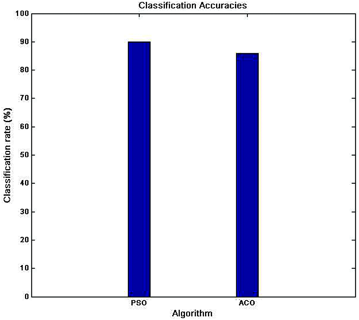
Figure 11: The recognition rate of PSO-MLP and ACO-MLP
4.3 Receiver Operating Characteristic Curves of GoogleNet and AlexNet
Receiver operating characteristic (ROC) curves estimate the performance of GoogleNet and AlexNet in breast cancer recognition by establishing a relationship between true positive rate and false positive rate. Fig. 12 shows the ROC curves of GoogleNet and AlexNet with a 0.0001 learning rate for Adam, RMSPROP, and SGDM. Both GoogleNet and AlexNet were found to have a stable learning process with slow convergence. Evaluation metrics, including the sensitivity of both DCNNs, reached 98–100%. A complete trade-off between the sensitivity and specificity of both the networks was found. GoogleNet and AlexNet act as perfect classifiers with the Adam optimizer, showing a true positive rate of one and false positive rate as zero.
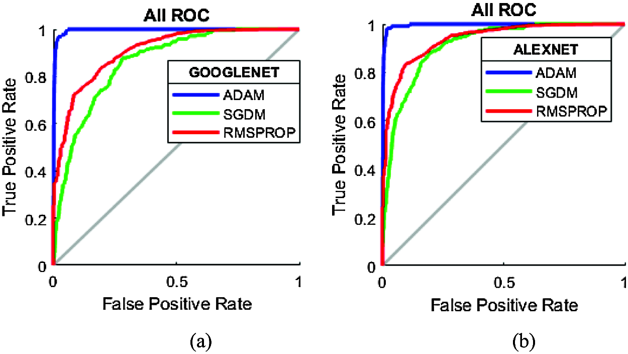
Figure 12: ROC curves for test data for 0.0001 learning rate: (a) GoogleNet; (b) AlexNet
In this paper, GoogleNet, a deep neural convolution network, was proposed for breast cancer recognition. The recognition process was carried out using a DDSM benchmark dataset containing normal, benign, and malignant cancer images. The performance of GoogleNet was assessed in terms of accuracy, loss rate, and runtime. The performance parameters were evaluated for different learning rates, namely 0.01, 0.001, and 0.0001, and with other optimizers such as Adam, RMSprop, and SGDM. DDSM images were preprocessed for breast and muscle identification, background removal, noise and blur removal using Wiener filter, contrast enhancement by CLAHE filter, and non-stationary noise removal using WPD by db3 wavelet. These methods produced a recognition accuracy of around 99% with the Adam optimizer and a learning rate of 0.0001. The average recognition rate was found to be high for a low learning rate. The loss rate was also low, and the runtime was 4.14 minutes. GoogleNet-based breast cancer recognition produces significantly high recognition compared to the PSO-MLP and ACO-MLP classifier, which use statistical features such as skewness, kurtosis, variance, entropy, contrast, correlation, energy, homogeneity, and mean extracted from the preprocessed image as input; accuracy levels of 90.21% and 86.14% were detected for the PSO-MLP and ACO-MLP classifiers, respectively. Further, DCNN-based GoogleNet was found to produce a runtime of 4.14 minutes, which is significantly lower than the run rates of 6.89 minutes and 8.54 minutes, respectively, for PSO-MLP and ACO-MLP. The performance of the GoogleNet-based breast cancer recognition system produces a lower loss rate of 0.1547 against the 0.1972 and 0.2234 produced by the PSO-MLP and ACO-MLP classifiers. Thus, the experimental results show that GoogleNet outperforms AlexNet, PSO-MLP, and ACO-MLP in state-of-the-art testing, with high accuracy, low loss rate, and runtime for breast cancer recognition when compared to the existing methods for the DDSM dataset.
Acknowledgement: The authors thank the management, director, principal, and Head of the CSE and EEE departments for permitting and facilitating this research.
Funding Statement: The authors received no specific funding for this study.
Conflicts of Interest: The authors declare that they have no conflicts of interest to report regarding the present study.
1. S. Tanini, A. D. Fisher, I. Meattini, S. Bianchi and J. Ristori, “Testosterone and breast cancer in transmen: Case reports, review of the literature, and clinical observation,” Clinical Breast Cancer, vol. 19, no. 2, pp. e271–e275, 2018. [Google Scholar]
2. R. L. Siegel, K. D. Miller and A. Jemal, “Cancer statistics,” CA Cancer Journal for Clinicians, vol. 68, no. 1, pp. 7–30, 2018. [Google Scholar]
3. S. A. Narod, “Tumour size predicts long-term survival among women with lymph node-positive breast cancer,” Current Oncology, vol. 19, no. 5, pp. 249–253, 2012. [Google Scholar]
4. A. B. Miller, C. Wall, C. J. Baines, P. Sun et al., “Twenty-five year follow-up for breast cancer incidence and mortality of the Canadian National Breast Screening Study: Randomised screening trial,” British Medical Journal, vol. 348, pp. 366, 2014. [Google Scholar]
5. R. M. Rangayyan, F. J. Ayres and J. E. L. Desautels, “A review of computer-aided diagnosis of breast cancer: Toward the detection of early signs,” Journal of the Franklin Institute, vol. 344, no. 3/4, pp. 312–348, 2007. [Google Scholar]
6. D. E. Goodman, L. C. Boggess and A. B. Watkins, “Artificial immune system classification of multiple-class problems,” Proceedings of the Artificial Neural Network in Engineering Systems, vol. 12, pp. 179–186, 2004. [Google Scholar]
7. J. R. Quinlan, “Improved use of continuous attributes in C4. 5,” Journal of Artificial Intelligence Research, vol. 4, pp. 77–90, 1996. [Google Scholar]
8. D. Nauck and R. Kruse, “Obtaining interpretable fuzzy classification rules from medical data,” Artificial Intelligence in Medicine, vol. 16, no. 2, pp. 149–169, 1999. [Google Scholar]
9. G. I. Salama, M. B. Abdelhalim and M. A. Zeid, “Breast cancer diagnosis on three different datasets using multi-classifiers,” International Journal of Computer and Information Technology, vol. 1, pp. 36–43, 2012. [Google Scholar]
10. H. J. Hamilton, N. Shan and N. Cercone, “RIAC: A rule induction algorithm based on approximate classification,” Technical Report, http://citeseerx.ist.psu.edu/viewdoc/download?doi=10.1.1.7.7768&rep=rep1&type=pdf, 1996. [Google Scholar]
11. K. Polat and S. Günes, “Breast cancer diagnosis using least square support vector machine,” Digital Signal Processing, vol. 17, no. 4, pp. 694–701, 2007. [Google Scholar]
12. A. Mert, N. Z. Kılıç, E. Bilgili and A. Akan, “Breast cancer detection with a reduced feature set,” Computational and Mathematical Methods in Medicine, pp. 1–11, Article ID 265138,2015. [Google Scholar]
13. J. Dheeba, N. A. Singh and S. T. Selvi, “Computer-aided detection of breast cancer on mammograms: A swarm intelligence optimized wavelet neural network approach,” Journal of Biomedical Informatics, vol. 49, no. 2, pp. 45–52, 2014. [Google Scholar]
14. A. M. Abdel-Zaher and A. M. Eldeib, “Breast cancer classification using deep belief networks,” Expert Systems with Applications, vol. 46, pp. 139–144, 2016. [Google Scholar]
15. M. Nilashi, O. Ibrahim, H. Ahmadi and L. Shahmoradi, “A knowledge-based system for breast cancer classification using fuzzy logic method,” Telematics and Informatics, vol. 34, no. 4, pp. 133–144, 2017. [Google Scholar]
16. S. Tiwari, “A variational framework for low-dose sinogram restoration,” Biomedical Engineering and Technology, vol. 24, no. 4, pp. 356–367, 2017. [Google Scholar]
17. Z. Gao, Y. Li, Y. Sun, J. Yang, H. Xiong et al., “Motion tracking of the carotid artery wall from ultrasound image sequences: A nonlinear state-space approach,” IEEE Transactions on Medical Imaging, vol. 37, no. 1, pp. 273–283, 2018. [Google Scholar]
18. Z. Gao, H. Xiong, X. Liu, H. Zhang, D. Ghista et al., “Robust estimation of carotid artery wall motion using the elasticity-based state-space approach,” Medical Image Analysis, vol. 37, no. 6, pp. 1–21, 2017. [Google Scholar]
19. C. Szegedy, W. Liu, Y. Jia, P. Sermanet, S. Reed et al., “Going deeper with convolutions,” in Proceeding of the IEEE Conference on Computer Vision and Pattern Recognition, Cornell University, pp. 1–9, 2015, arXiv:1409.4842. [Google Scholar]
20. Y. Yuan and M. Meng, “Deep learning for polyp recognition in wireless capsule endoscopy images,” Medical Physics, vol. 44, no. 4, pp. 1379–1389, 2017. [Google Scholar]
21. S. Wan, Y. Liang and Y. Zhang, “Deep convolutional neural networks for diabetic retinopathy detection by image classification,” Computers and Electrical Engineering, vol. 72, no. 10, pp. 274–282, 2018. [Google Scholar]
22. H. Cho, Y. Kim, E. Lee, D. Choi, Y. Lee et al., “Basic enhancement strategies when using Bayesian optimization for hyperparameter tuning of deep neural networks,” IEEE Access, Special Section on Scalable Deep Learning for Big Data, vol. 8, pp. 52588–52608, 2020. [Google Scholar]
23. R. Mendes, P. Cortez, M. Rocha and J. Neves, “Particle swarms for feed-forward neural network training,” in Proc. of the 2002 Int. Joint Conf. on Neural Networks, Honolulu, HI, USA, pp. 1895–1899, 2002, INSPEC Accession Number: 7328548. [Google Scholar]
24. C. Blum and K. Socha, “Training feed-forward neural networks with ant colony optimization: An application to pattern classification,” in Proc. of the Int. Conf. on Hybrid Intelligent System, Rio de Janeiro, Brazil, pp. 233–238, 2005. [Google Scholar]
 | This work is licensed under a Creative Commons Attribution 4.0 International License, which permits unrestricted use, distribution, and reproduction in any medium, provided the original work is properly cited. |