Intelligent Automation & Soft Computing DOI:10.32604/iasc.2022.020435
Article

Robustness Convergence for Iterative Learning Tracking Control Applied to Repetitfs Systems

Ben Attia Selma*, Ouerfelli Houssem Eddine and Salhi Salah

Laboratory of Analysis, Conception and Control of Systems (LACCS), University of Tunis El Manar, Tunis, 1002, Tunisia
*Corresponding Author: Ben Attia Selma. Email: benattiaselma@gmail.com
Received: 24 May 2021; Accepted: 22 July 2021

Abstract: This study addressed sufficient conditions for the robust monotonic convergence of repetitive discrete-time linear parameter varying systems, with the parameter variation rate bound. The learning law under consideration is an anticipatory iterative learning control. Of particular interest in this study is that the iterations can eliminate the influence of disturbances. Based on a simple quadratic performance function, a sufficient condition for the proposed learning algorithm is presented in terms of linear matrix inequality (LMI) by imposing a polytopic structure on the Lyapunov matrix. The set of LMIs to be determined considers the bounds on the rate of variation of the scheduling parameter. The control law designs polynomial ILC by constructing a sequence of control inputs to a discrete-time R-LPV system, producing an iterative dynamic for the R-LPV system with respect to the polytopic structure for uncertain parameters. Numerical simulations were performed to demonstrate the benefits of the proposed technique.

Keywords: ILC control; quadratic approach; LMI; repetitive LPV systems; output disturbance; robust control

1  Introduction

Repetitive linear parameter varying processes (R-LPVs) are a distinct class of 2D systems [1,2] (i.e., information propagation in two independent directions) of both system theoretic and application interest whose unique characteristic is a series of sweeps, termed “passes,” through a set of dynamics defined over a fixed finite duration known as the “pass length,” and many articles have been published [3,4]. On each pass, an output, called the “parameter varying pass profile,” is produced, which acts as a forcing function on, and, hence, contributes to, the dynamics of the next pass profile [5,6].

Physical examples of these processes include long-wall coal-cutting and metal-rolling operations [7]. In recent years, applications have arisen, where adopting a repetitive parameter varying process setting for analysis has distinct advantages over alternatives. An example of these algorithmic applications is iterative algorithms for solving nonlinear dynamic optimal stabilization problems based on the maximum principle [8], where the use of the repetitive process setting provides the basis for the development of extremely reliable and efficient iterative solution algorithms [9–11].

In particular, iterative learning control schemes provide one approach for controlling systems operating in a repetitive parameter varying (or pass-to-pass) mode with the requirement that a reference trajectory yk (t) defined over a finite interval 0 ≤ t ≤ T be followed with high precision [12,13]. In this case, a repetitive process setting for analysis provides a stability theory that, unlike many alternatives, enables the design to meet pass-to-pass error convergence and control of the along-the-pass dynamics.

The problem considered in this study is similar to robust iterative learning control (ILC) for linear discrete-time R-LPV systems [14,15] with a prescribed bound on the rate of parameter variation [16–20]. In this regard, ILC has attracted attention for the past two decades. A 2D system theory view of ILC has been considered, and the tracking problems generally treated under the ILC framework must have some 2D properties. With the help of a delay operator in the time domain (standard Z-transformation), the dynamics of linear discrete-time systems are converted into a dynamic process in the iteration domain. This extension can be applied to time R-LPV systems, input variables, output variables, and errors. Based on this idea, the tracking problem and the stabilization problem of R-LPV systems is a topic that has been studied extensively, to the best of the authors’ knowledge. However, basic control problems, such as stability and stabilization, can be relatively easily extended to involve robustness analysis and more control performance specifications using H∞ norms. Therefore, robust monotonic convergence (RMC) is formulated in terms of a set of linear matrix inequalities (LMIs), while the learning gains can be determined directly by solving the LMIs. The stability analysis shows that the output error l2 norm has RMC as the learning process proceeds from one trial to the next.

The remainder of this paper is organized as follows. Section 2 provides a brief description of the problem formulation and a discussion of the control objective. In Section 3, the idea that the convergence conditions for the polynomial control law design ILC based on the bounded real lemma (BRL) approach produce a monotonic convergence error at iteration for an LPV repetitive system with varying bounded parameters is described. In Section 4, the stability analysis of the system and sufficient conditions for the existence of a stabilizing polynomial ILC controller are derived in terms of a set of matrix inequalities. In Section 5, a new approach for a system to achieve optimal noise attenuation using the ILC control problem for R-LPV systems with output disturbance is discussed. In Section 6, numerical examples are presented to illustrate the feasibility and effectiveness of the design algorithms in this study. Finally, the conclusions of this study are presented in Section 7.

Throughout this work, the null matrix and the identity matrix with appropriate dimensions are denoted by 0 and I, respectively. In large matrix expressions, the symbol * replaces the terms that are induced by symmetry, ‖ ‖ denotes the induced operator norm, and Z is a z transform. The expression sym(M) represents a symmetric matrix M + MT, and diag{x, y} denotes the diagonal matrix obtained from vectors or matrices x, y.

2  Problem Statement

2.1 System Description

The following discrete linear repetitive parameter varying system is considered over t∈[0,T],k∈Z+

{xk+1(t+1)=A(θ(t))xk+1(t)+B(θ(t))vk+1(t)yk+1(t)=C(θ(t))xk+1(t)xk(0)=x0t∈0,…,T (1)

where k is the iteration number, which denotes the kth repetitive operation of the system, and xk+1(t) ∈ ℝn, and yk+1(t) ∈ ℝl are the state, input, and output variables, respectively. Moreover, x0 is the initial condition for each iteration. It is assumed that the dynamic matrices A(θ(t)), B(θ(t)), C(θ(t)) are dependent on the parameters θi(t), i.e.,

A(θ(t))=∑i=1Nθi(t)Ai;B(θ(t))=∑i=1Nθi(t)Bi;C(θ(t))=∑i=1Nθi(t)Ci (2)

where Ai, Bi, Ci, Di are a constant matrix i = (1, …, N).

The time-varying parameter θ(t) varies in a polytope given by θ(t) ∈ ΛN, where

ΛN:={θ∈Rn:∑i=1Nθi(t)=1,θi≥0,i=1,….N} (3)

where N is the number of vertices of the polytope.

If a control law of the following form exists over t ∈ [0, T] and k ∈ ℤ+,

vk+1(t)=uk+1(t)+L(θ(t))xk+1(t) (4)

where L(θ(t))=∑m=1NθmLm is the parameter varying gain for each polytope,

By applying the control law in Eq. (4) to the system in Eq. (1), the following state space is obtained.

{xk+1(t+1)=Acl(θ(t))xk+1(t)+B(θ(t))uk+1(t)yk+1(t)=C(θ(t))xk+1(t) (5)

where Acl(θ(t)) = A(θ(t)) + B(θ(t)) L(θ(t))

For all t ≥ 0, the rate of variation of the parameters is defined by:

Δθi(t)=θi(t+1)−θi(t),i=1,…,N (6)

Is assumed to be limited by an a priori known bound b such that: − b ≤ Δθi(t) ≤ b  i = 1, …, N In this work, a specific case of polytopic discrete-time R-LPV systems with known bounds on the rate of variation of the parameters Δθi(t) is proposed that is well defined at all times and satisfies the Lemma 1.

Lemma 1. If the uncertain parameter Δθi(t) belongs to the set given by Eq. (6) and satisfies previous Equation, then its time derivative can be written as:

Δθi(t)=b(σj1−βj2) (7)

where σj1 and βj2 verify

σ(t)∈ΛN;ΛN:={σ∈Rn:∑j1=1Nσj1=1,σj1≥0} (8)

β(t)∈ΛN;ΛN:={β∈Rn:∑j2=1Nβj2=1,βj2≥0} (9)

2.2 Control Objective

The following assumption is considered for the R-LPV system in Eq. (1).

A1. The desired output yd(t), t = 1, …, T is given a priori over the same time duration, and it is assumed that the initial resetting condition is satisfied, i.e., yk(0) = yd(0).

It follows from Eq. (5) that the Z-transform of the output is of the form

Xk+1(z) = (zI − Acl (θ)) −1B(θ) Uk+1(z) when

Yk+1(z)=C(θ)(zI−Acl(θ))−1B(θ)Uk+1(z)=G(z)Uk+1(z) (10)

where G(z) = C(θ) (zI − Acl (θ)) −1B(θ)

A2. The initial state remains the same at each iteration, i.e., xk(0)=0,∀k=1,2,…

For any given assumptions A1 and A2, one desirable objective in ILC is that yk(t) converges monotonically to yd (t) when k tends to infinity for all t within the time interval [0, T]. This can guarantee reasonable transients during the learning process. In the sense of the ℓ2,[0,T] norm, this objective can be transformed by considering the index.

J(γ,k)=∑t=1N[ek+1T(t)ek+1(t)−γ2ekT(t)ek(t)] (11)

where γ > 0 is the prescribed scalar, and ek(t)is the tracking error at the kth iteration, expressed as

ek(t)=yd(t)−yk(t) (12)

The norm error ‖ek(t)‖2[0,T] can be guaranteed to converge monotonically along the iteration axis k if J(γ) < 0 holds for any γ ∈ ]0, 1[. With this fact, the objective can be given as follows.

The objective of this study is to present LMI conditions to ensure the monotonic convergence of ILC by considering the performance index J(γ, k) of Eq. (16) and applying the BRL from the robust H∞ control theory.

To achieve this objective, it should be noted that, for a prescribed scalar, γ, J(γ) can be transformed as the performance index defined for the system.

Ek+1(z)=H(z)Ek(z) (13)

where Ek(z) = Z[ek(t)], and H(z) is a transfer function matrix to be determined.

Once the system in Eq. (18) is established, ‖G‖∞ < γ can be used to guarantee that J(γ) < 0.

Moreover, there exist matrices Acl(θ), Bcl(θ), Ccl(θ), Dcl(θ) such that H(z) is expressed in the form

H(z)=Ccl(θ)(zI−Acl(θ))−1Bcl(θ)+Dcl(θ):=[Acl(θ)Ccl(θ)|Bcl(θ)Dcl(θ)] (14)

Using the fact that ‖Ek(z)‖2=‖ek(t)‖2 yields: ‖ek+1(t)‖2<‖H‖2‖ek(t)‖2 (15)

which leads to: ‖ek(t)‖2<‖H‖∞k‖e0(t)‖2 (16)

Hence, it can be derived that, if ‖H(z)‖∞ < γ, γ ∈ [0, 1) holds, then limk→∞⁡‖ek(t)‖2=0 (monotonic convergence in the sense of the l2 norm). This implies that, although the tracking error over the finite time interval [0, T] is considered in ILC, the monotonic convergence of ‖ek(t)‖2 can also be guaranteed when ‖H(z)‖∞ < γ is used to obtain the negative performance index J(γ) < 0.

3  Design for ILC-Tracking Control

Now, the polynomial ILC law is as follows.

Uk+1(z)=Uk(z)+K(θ,z)Ek(z) (17)

where: K(θ,z)=∑q=0r∑mNθmKm,rzq

In which the Z-transform Ek(z) = Z[ek(t)], Km,r is a polynomial learning varying gain matrix to be designed, and r is the degree of K(θ, z).

According to the developments in Section 2.2, it is straightforward to derive an H∞ condition for the monotonic convergence of the ILC system in Eqs. (5) and (17). When Ek is subtracted from Ek+1 and Eqs. (10) and (17) are inserted, one obtains

Ek+1(z)−Ek(z)=−(Yk+1(z)−Yk(z))=−G(z)(Uk+1(z)−Uk(z))=−G(z)K(θ,z)Ek(z) (18)

which leads to:

Ek+1(z)=(I−G(z)K(θ,z))Ek(z) (19)

Comparing Eq. (19) with Eq. (13) yields:

H(z)=(I−G(z)K(θ,z)) (20)

Lemma 2. Consider the ILC system in Eqs. (1) and (17). If K(θ, z) is designed such that ‖I − G(z) K(θ, z)‖ < γ, γ ∈ (0, 1] is satisfied, then the tracking error ek(t) converges monotonically to zero when k tends to infinity in the sense of the l2,[0,T] norm. According to the previous developments, it is straightforward to derive a condition for the monotonic convergence of ILC–R-LPV system in Eqs. (1) and (17).

From Eq. (20), one obtains:

H(z)=I−C(θ)(zI−Acl(θ))−1B(θ)∑q=0rKq(θ)zq (21)

The relative degree of the polynomial regulator r = 1, and, based on Eq. (21), one obtains this result:

H(z)=I−C(θ)(zI−Acl(θ))−1B(θ)[K0(θ)+zK1(θ)] (22)

Using the fact that:

z(zI−Acl(θ))−1=I+Acl(θ)(zI−Acl(θ))−1 (23)

and respecting Eq. (23),

H(z)=I−C(θ)(zI−Acl(θ))−1B(θ)K0(θ)−C(θ)(zI−Acl(θ))−1B(θ)zK1(θ)=I−C(θ)(zI−Acl(θ))−1B(θ)K0(θ)−C(θ)z(zI−Acl(θ))−1⏟I+Acl(θ)(zI−Acl(θ))−1B(θ)K1(θ) (24)

4  LMI Condition

In this section, the LMI conditions are presented to ensure the monotonic convergence of the ILC–R-LPV system by considering the performance index J(γ) and applying the BRL from the robust H∞ control theory.

Theorem 1. If one considers the R-LPV system in Eq. (1) and the ILC law with r = 1, then the tracking error robustly converges monotonically to zero when k tends to infinity in the sense of the l2,[0,T] norm if there exist scalars γ > 0 and N symmetric positive matrices Pi > 0 and the appropriate matrices Gj1m, Rj1mK1m, K0m that satisfy the following LMIs:

[−b(Pj1−Pj2)−Pi∗∗∗∗0−Pi∗∗∗(BiK0,m)T0−I∗∗0−CiPiI−Cj1BiK1,m−γ2I∗Gj1TAiT+Nm,j1TBiTPiTBiK1,m0−Gj1−Gj1T]<0 (25)

In addition, Lm=Nj,mGj1−1 .

Proof 2: Applying the BRL [18] to Eq. (24), it follows that a sufficient condition for ‖H(z)‖∞ < γ is the existence of a positive definite solution P(θ(t)) > 0 to the following inequality:

[−P(θ(t+1))∗P(θ(t))(Acl(θ(t)))T−P(θ(t))(B(θ)K0(θ)+Acl(θ(t))B(θ)K1(θ))T00−C(θ)P(θ(t))∗∗∗∗−I∗I−C(θ)B(θ)K1(θ)−γ2I]<0 (26)

Subsequently, the so-called “relaxation method” discussed in a previous report [21] is introduced to decouple the Lyapunov variable from the system matrices to provide more design freedom. The LMI in Eq. (24) can be written as:

[−P(θ(t+1))∗0−P(θ(t))(B(θ(t))K0(θ(t)))T00−C(θ(t))P(θ(t))G(θ(t))TAcl(θ(t))TP(θ(t))T∗∗∗∗∗∗−I∗∗Dcl(θ(t))−γ2I∗B(θ(t))K1(θ(t))0−G(θ(t))−G(θ(t))T]<0 (27)

The parameter-dependent LMI conditions in Eq. (27) must be evaluated for all θ(t) in the unit simplex ΛN, which leads to an infinite-dimensional problem. By imposing an affine parameter-dependent structure on the Lyapunov matrix P(θ(t)), such that:

P(θ(t))=∑i=1Nθi(t)Pi (28)

and Δθi(t) given by Eq. (6) replaces Eq. (6) into Eq. (28), one obtains

P(Δθ(t))=∑i=1Nθi(t+1)Pi−∑i=1Nθi(t)Pi (29)

Using Eqs. (8) and (29), it can be shown that

P(θ(t+1))=∑i=1NΔθi(t)Pi+∑i=1Nθi(t)Pi=b(P(σ(t))−P(β(t)))+P(θ(t)) (30)

where σj1(t),βj2(t) both have polytopic structures, as in Eqs. (9) and (10). Thus, Eq. (27) can be written as

[−b(P(σ(t))−P(β(t)))−P(θ(t))∗0−P(θ(t))(B(θ(t))K0(θ(t)))T00−C(θ(t))P(θ(t))G(θ(t))TAcl(θ(t))TP(θ(t))T∗∗∗∗∗∗−I∗∗Dcl(θ(t))−γ2I∗B(θ(t))K1(θ(t))0(−G(θ(t))−G(θ(t))T)]<0 (31)

Then, assuming that θm(t),θi(t),θj1(t),σj1(t),βj2(t) that evolve in the polytopes defined by Eqs. (3)–(9) and (10) holds, one rewrites the LMI in Eq. (31) as

[−b(Pj1−Pj2)−Pi∗∗∗∗0−Pi∗∗∗(BiK0,m)T0−I∗∗0−CiPiI−Cj1BiK1,m−γ2I∗Gj1T(Ai+BiLm)TPiTBiK1,m0−Gj1−Gj1T]<0 (32)

Using the change of variable LmGj1=Nj,m , the LMI in Eq. (42) needs to Eq. (30).

5  Robust Control of R-LPV Systems with Output Disturbances

This section starts with a problem of gain-scheduled H∞control formulation. The associated robust stability condition with a tracking error of zero is developed. The class of R-LPV discrete-time linear systems with output disturbance is considered.

{xk+1(t+1)=Acl(θ(t))xk+1(t)+B(θ(t))uk+1(t)yk+1(t)=C(θ(t))xk+1(t)+Bw(θ(t))wk+1(t)zk+1(t)=ek(t)+Dw(θ(t))wk+1(t) (33)

where (Acl(θ(t)), B(θ(t)), C(θ(t)), Bw(θ(t)), Dw(θ(t))) are the matrices describing the system in the state space, wk+1(t) ∈ ℝl×1 represents any repeating disturbance written as an equivalent output disturbance, and zk+1(t) is the measured output. The fundamental aim is to make yk+1(t) converge to yd(t) for all k tending to infinity and to guarantee that the design of a control law continuously monitors the performance of the studied system and changes the commands as necessary to stay on track.

It follows from Eq. (33) that the Z-transform of the output is of the form

Yk+1(z)=G(z)Uk+1(z)+dWk+1(z) (34)

where d denotes the disturbance vectors and describes the contribution from external sources in the current trial. From Eqs. (17) and (33),

Ek+1(z)−Ek(z)=−(Yk+1(z)−Yk(z))=−G(z)(Uk+1(z)−Uk(z))+d(Wk+1(z)−Wk(z))=−G(z)K(θ,z)Ek(z)+d(Wk+1(z)−Wk(z)) (35)

This leads to

Ek+1(z)=(I−G(z)K(θ,z))Ek(z)+d(Wk+1(z)−Wk(z)) (36)

Using Eq. (36) and respecting Eq. (20),

Ek+1(z)=H(z)Ek(z)+d(ΔWk+1(z)) (37)

It is easy to verify that parameter uncertainty in a linear setting can often be modeled as Fig. 1.

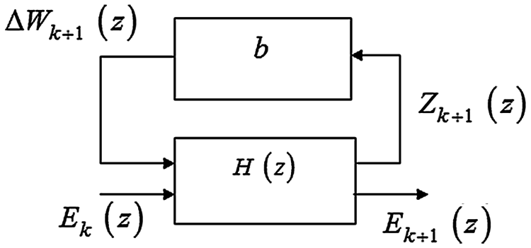
Figure 1: Uncertain model

Introducing ηk+1(t) as the state vector, which is related to the previous system in Eq. (37), the following state space representation is obtained:

T(θ(t)):{[ηk+1(t+1)ek+1(t)_zk+1(t)]=[Acl(θ(t))(B(θ)K0(θ)+Acl(θ)B(θ)K1(θ))−C(θ)I−C(θ)B(θ)K1(θ)0I][ηk+1(t)ek(t)]+[0Bw(θ(t))Dw(θ(t))]Δwk+1(t);ηk+1(0)=0,k=0,1,... (38)

For a prescribed scalar, γ, J(γ) can be transformed as the performance index defined for the system.

First, x¯k+1(t)=ηk+1(t+1),y¯k(t)=[e¯k+1(t)z¯k+1(t)]T (39)

and

A¯(θ(t))=Acl(θ(t)),B¯(θ(t))=[(B(θ)K0(θ)+Acl(θ)B(θ)K1(θ))0]C¯(θ(t))=[−C(θ)0],D¯(θ(t))=[I−C(θ)B(θ)K1(θ)Bw(θ(t))IDw(θ(t))] (40)

Then, from Eqs. (39) and (40), given this repetitive single-input multi-output model,

{x¯k+1(t+1)=A¯(θ(t))x¯k+1(t)+B¯(θ(t))wk+1(t)y¯k+1(t)=C¯(θ(t))x¯k+1(t)+D¯(θ(t))wk+1(t) (41)

This 1D equivalent model was developed in previous research [22,23], and here it is only necessary to give the final construction. Here, x¯k+1(t) represents the input state vector, y¯k+1(t) is the output vector, wk+1(t) ∈ ℝq is the exogenous input that belongsl2{[0, ∞), [0, ∞)}, and zk+1(t) is the controlled output. Moreover, A¯(θ(t)) , B¯(θ(t)) , C¯(θ(t)) , and D¯(θ(t)) are constant matrices with appropriate dimensions. and the transfer function for Eq. (41) is T(z)=C¯(θ(t))(zI−A¯(θ(t)))B¯(θ(t))+D¯(θ(t)) .

Theorem 2. The R-LPV system in Eq. (1) and the ILC law with r = 1 are considered. The tracking error robustly converges monotonically to zero when k tends to infinity in the sense of the l2,[0,T] norm if there exist scalars γ > 0 and N symmetric positive matrices Pi > 0, and the appropriate matrices Gj1m, Rj1mK1m, K0m that satisfy the following LMIs:

[6pt−b(Pj1−Pj2)−Pi0BiK0,m6pt∗−Pi0∗∗−I∗∗∗∗∗∗∗∗∗∗∗∗8pt000AiGj1+BiRm,j10−PiCj1T0Pi8pt0I−Cj1BiK1,mI(BiK1,m)T8pt−IBi,wTDi,wT0∗−γ2I00∗∗−γ2I0∗∗∗−Gj1T−Gj1]<0 (42)

In addition, Lm=Nj,mGj1−1 .

Proof 3. Applying the BRL [18] to Eq. (38), it follows immediately that a sufficient condition for ‖H(z)‖∞ < γ is the existence of a positive definite solution P(θ(t)) > 0 to the following inequality:

[−P1(θ(t+1))Acl(θ(t))P1(θ(t)){B(θ(t))K0(θ(t))+Acl(θ(t))B(θ(t))K1(θ(t))}∗−P1(θ(t+1))0∗∗−I∗∗∗∗∗∗∗∗∗0000−P1(θ(t))CT(θ(t))00(I−C(θ(t))B(θ(t))K1(θ(t)))I−IBwT(θ(t))DwT(θ(t))∗−γ2I0∗∗−γ2I]<0 (43)

in much the same way, leading to

[−P(θ(t+1))0B(θ(t))K0(θ(t))∗−P(θ(t))0∗∗−I∗∗∗∗∗∗∗∗∗0000−P1(θ(t))CT(θ(t))00(I−C(θ(t))B(θ(t))K1(θ(t)))I−IBwT(θ(t))DwT(θ(t))∗−γ2I0∗∗−γ2I]+{[Acl(θ(t))00000][0P1(θ(t))(B(θ(t))K1(θ(t)))T000]+sym(..)}<0 (44)

which is transformed using the projection lemma used in a previous study and the Schur complement technique. It follows that

[−P(θ(t+1))0B(θ(t))K0(θ(t))∗−P(θ(t))0∗∗−I∗∗∗∗∗∗∗∗∗∗∗∗000Acl(θ(t))G(θ(t))0−P1(θ(t))CT(θ(t))0P(θ(t))0(I−C(θ(t))B(θ(t))K1(θ(t)))I(B(θ(t))K1(θ(t)))T−IBwT(θ(t))DwT(θ(t))0∗−γ2I00∗∗−γ2I0∗∗∗−GT(θ(t))−G(θ(t))]<0 (45)

The LMI in Eq. (45) gives polytopic structures that come directly from Section 4, so that the proof will be almost omitted. Given P(θ(t)) = X−1(θ(t)), one obtains Eq. (43).

6  Simulation Results

6.1 Application to Printing Systems

The effectiveness of the proposed method was demonstrated by simulation. MATLAB software was used for the simulation. The wide-format printer and paper positioning are shown in Figs. 2 and 3. The aim of this system was to correct quickly the angular offset paper sheets that pass through the unit at high speeds. During this motion, the inertia of the sheets changes the motors, which are modeled with LPV dynamics.

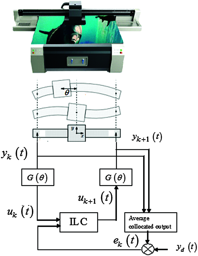
Figure 2: Dynamics of an industrial flat-bed printer dependent on its configuration

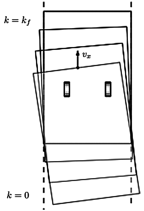
Figure 3: Inertia of the sheet: the pinches change, which is modeled as LPV dynamics

6.2 Description

The accurate positioning of the carriage in the y-direction is hampered by a resonance mode that varies as a function of its x-position, as schematically shown in Figs. 2 and 3. A symmetric force is applied to uk(t), and the output is the average of the collocated memory output y∞=12(yk+yk+1) .

A simplified polytopic LPV model is given by

where δ ∈ ℝ+ is a given nonnegative scalar. These system matrices were borrowed from a prior report [24,25].

6.3 Simulation of Comparison

The problem considered here is the design of an iterative learning controller that stabilizes the R-LPV system. The result obtained using Theorem 1 is compared with the three methods developed in previous studies and summarized in Tab. 1. The R-LPV system is characterized by the number of vertices of the polytope (N), system order (n), number of inputs (m), and number of outputs (l). For fixed values of (N, n, m, l), 100 R-LPV systems of the form in Eq. (1) were generated. Therefore, the purpose was to design an ILC controller using four methods in the form of Eq. (22) such that the closed system is robust and stable, and the output system converges to the desired trajectory.

Method 1 uses switching ILC control in Theorem 2.

Method 2 uses the method developed in a previous study [1].

Method 3 uses the method developed in another study [6].

Method 4 uses a method developed previously [8].

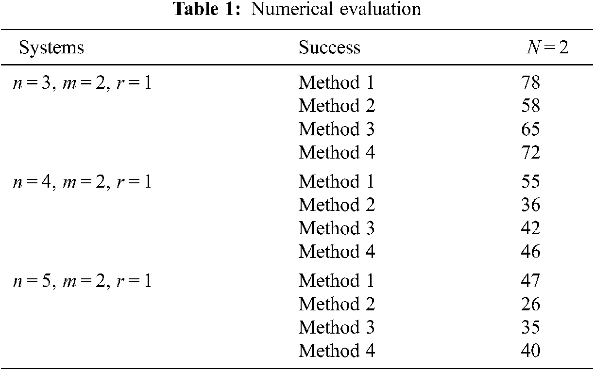
By using the MATLAB LMI Control Toolbox to check the feasibility of the LMI conditions, a counter (Success Method 1, Success Method 2, Success Method 3, and Success Method 4) was introduced, which is increased if the corresponding method succeeds in providing an ILC-tracking control.

The contribution of this study is the combination of a specific case of polytopic discrete-time R-LPV systems with known bounds on the rate of variation parameters Δθi(t) with robust stability by applying ILC control.

The aim was to determine the maximum limits of stability in the plane (δ, b) from one side (based on Theorem 1) such that the system is robust and monotonically stabilized by varying learning gains — the LMIs in Eq. (30) are feasible — and to guarantee the upper bound of the real parameter γ. The result obtained using Theorem 1 was compared with the method developed in other research and is summarized in Tab. 2.

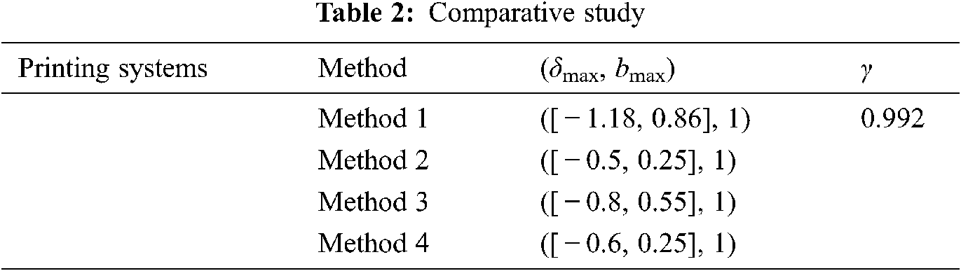
The computational results show that the condition in Theorem 1 is less conservative than the results given in the other methods.

Fig. 4 shows the resulting maximum allowed bound bmax on the rate of variation for the different control designs as a function of the scalar stabilizability regions by the maximum variation of the parameter. The gain parameters obtained by Theorem 1 (optimization problem) are as follows:

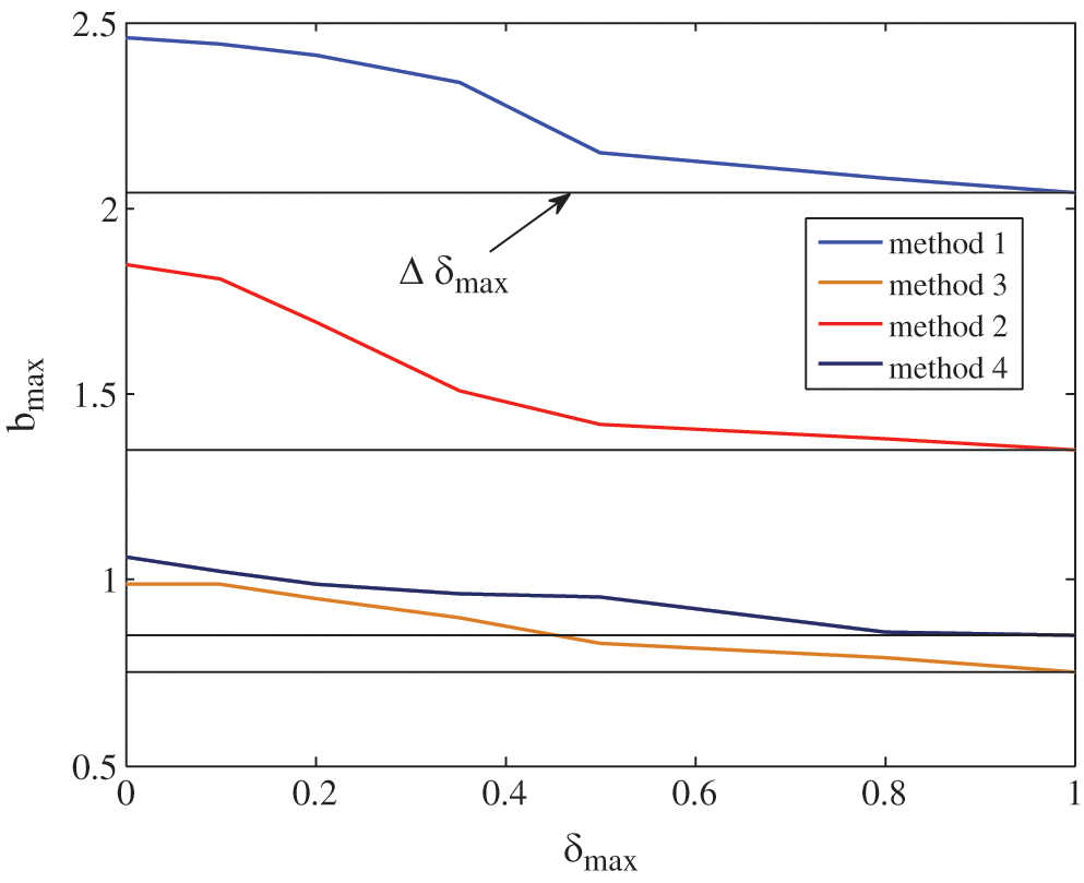
Figure 4: Stabilizability regions as a function of the plane (δ, b)

To check the performance achieved using the new design procedure, b is fixed to b = 1. Fig. 5 shows the achieved upper bound γmax = 0.998 of the closed-loop system in Eq. (29) as a function of the allowed bound on the rate of variation.

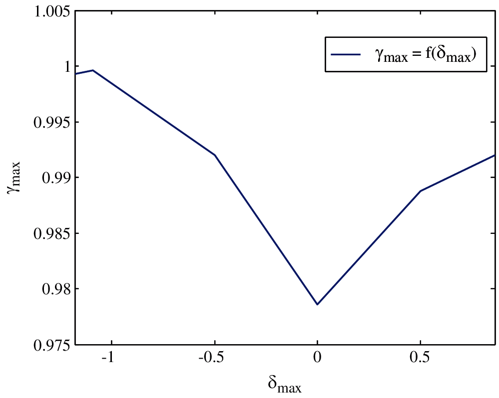
Figure 5: Guaranteed upper bounded γ as a function of uncertain parameter δ

6.4 Monotonic Tracking Error

In this study, the linear system in Eq. (16) was considered. The desired trajectory was set as

First, the resulting ILC process can be guaranteed with its tracking error converging to zero along the iteration and time. Figs. 6 and 7 show the time evolution of the output error ek(t) and the output system profiles yk(t) successively at the maximum value of δmax = 0.86, b = 1.

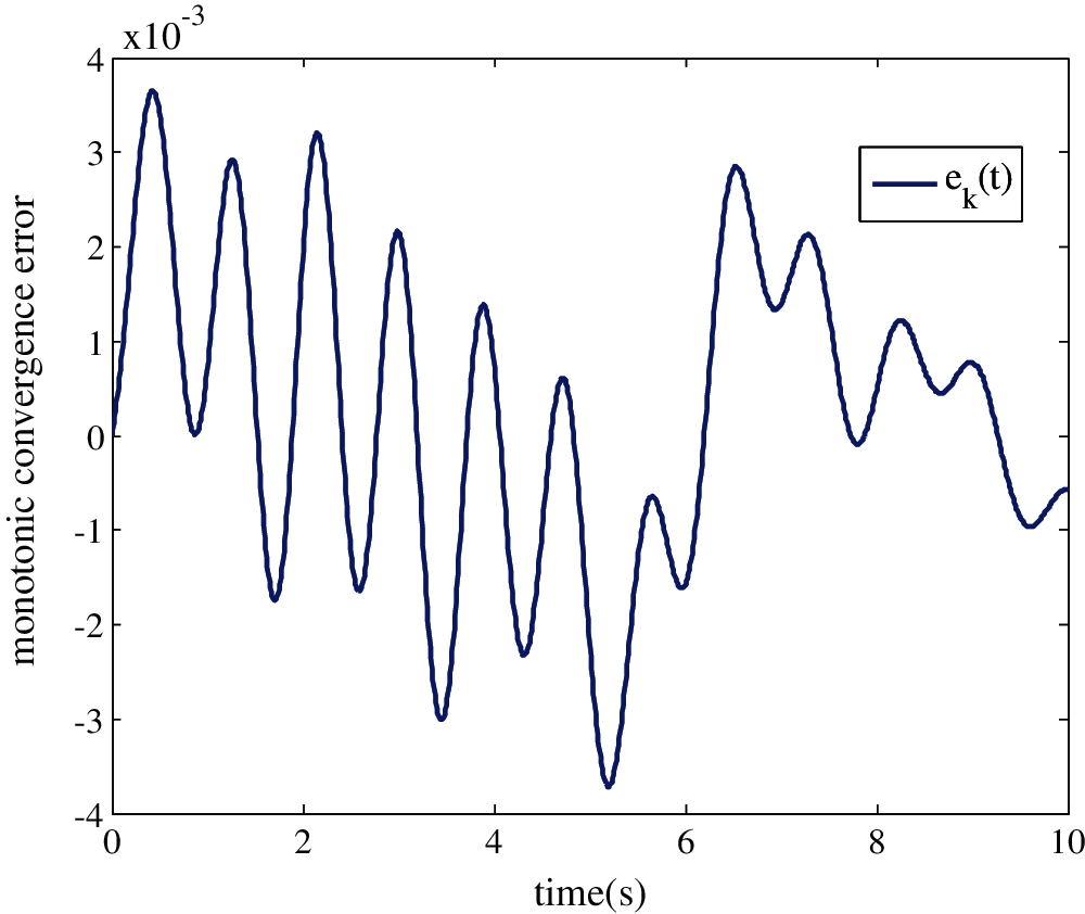
Figure 6: Evolution of the error ek(t) to zero for the maximum value of δmax after 10 iterations

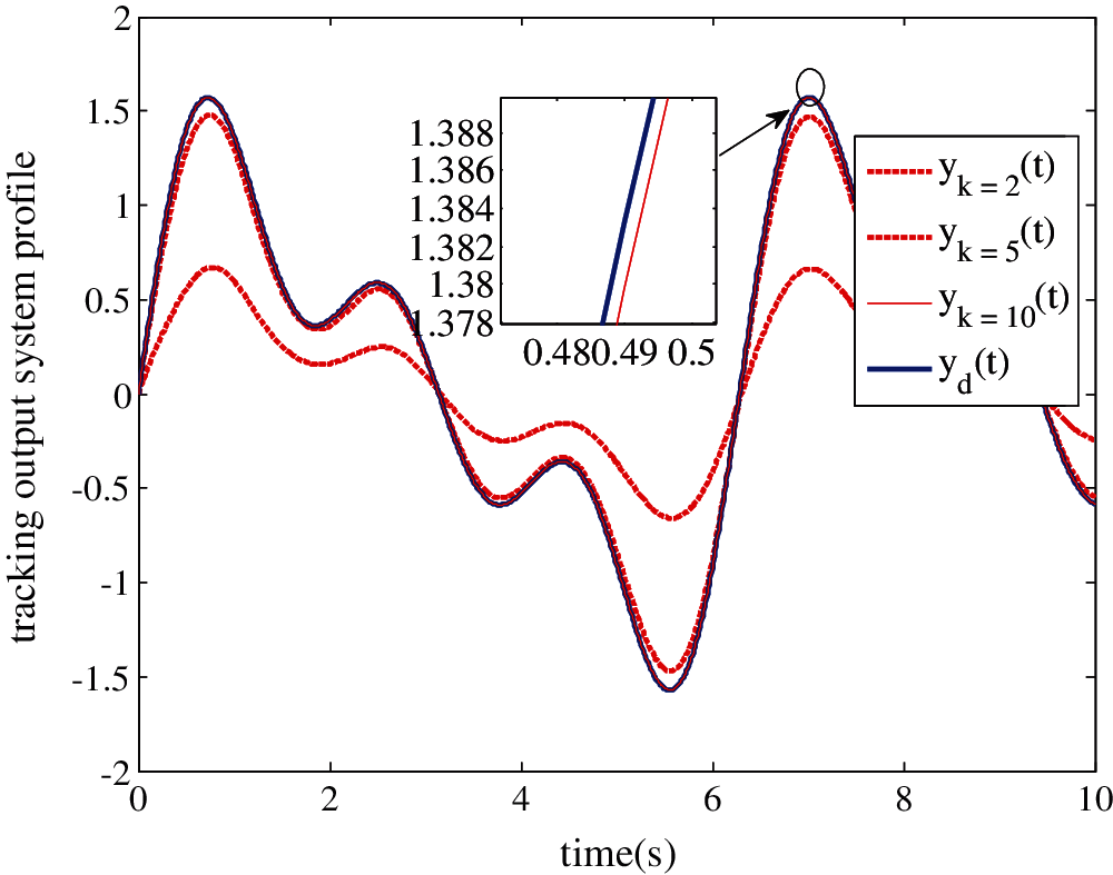
Figure 7: Evolution of the output trajectory yk(t) to desired trajectory yd(t). for the maximum value of δmax after 10 iterations

Remark. The feasibility of the studied problem with a maximum value of (δmax, bmax) requires a certain number of iterations to converge on the desired output. However, the influence of the two parameters (δ, b) on the rapidity of the monotonic convergence of the ILC controller.

First, b is fixed to be bmax = 1 and for different values of the uncertain varying parameter δ to check the influence of δ on the convergence of error at five iterations.

Fig. 8 shows that using the maximum value of δmax = 0.55 found in a previous report [6], one can guarantee the monotonic convergence of error at the minimum number of iterations and guarantee a very important tracking between yk(t), yd(t)—hence, the efficiency of the algorithm shown in Theorem 1.

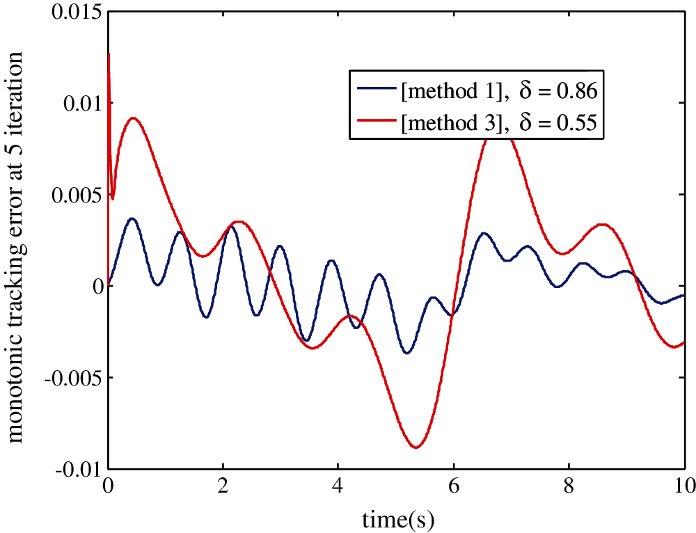
Figure 8: Output error convergence at five iterations as a function of the uncertain varying parameter δ, b = 1

However, Fig. 9 shows evolution of the tracking error with respect to the allowed bound b. Now, δ is fixed to be δmax = 0.86. To check the influence of the bound b on the limited iteration number, different cases are considered: b = {0.25, 0.8, 1}. Thus, the resulting ILC process can be tested with its tracking error converging to zero over five iterations.

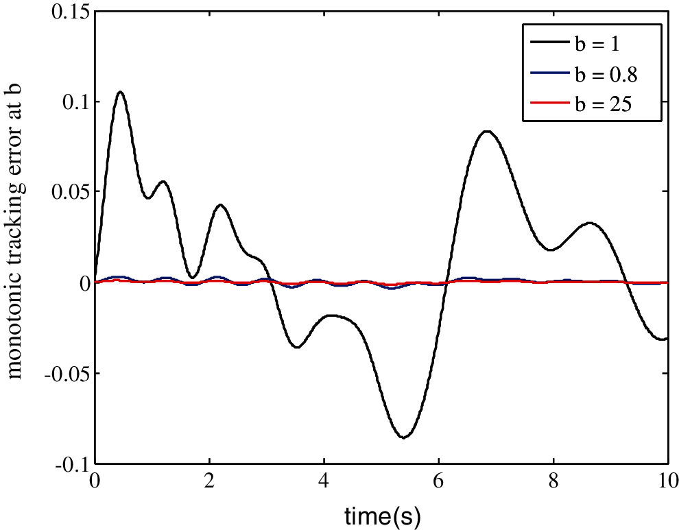
Figure 9: Output error convergence at five iterations as a function of the allowed bound b, δmax = 0.86

The control effort required for this study is shown in Fig. 9, where, as the speed of varying uncertain parameter b increases, the output error between iterations increases. Thus, from the upper bound of bmax, the system requires more iterations, so the error converges to zero.

7  Conclusion

In this study, the problem of polynomial ILC-tracking control induced by the BRL was discussed for a class of linear R-LPV systems with a prescribed bound on the rate of parameter variation. The control law designs polynomial ILC by constructing a sequence of control inputs to a discrete-time R-LPV system, producing an iterative dynamic for the R-LPV system with respect to the polytopic structure for uncertain parameters. This can guarantee the monotonic convergence error of the closed-loop R-LPV system. The ILC algorithm should be studied when there are disturbances in the system, and it was shown that the choice in the ILC algorithm depends highly on the type of disturbance. Sufficient conditions for the existence of such a controller were formulated in terms of a set of LMIs. A numerical example was provided to illustrate the effectiveness of the proposed method.

Funding Statement: The authors received no specific funding for this study.

Conflicts of Interest: The authors declare that they have no conflicts of interest to report regarding the present study.

This work is licensed under a Creative Commons Attribution 4.0 International License, which permits unrestricted use, distribution, and reproduction in any medium, provided the original work is properly cited.