Intelligent Automation & Soft Computing DOI:10.32604/iasc.2022.022231
Article

Forecasting of Trend-Cycle Time Series Using Hybrid Model Linear Regression

N. Ashwini1,*, V. Nagaveni2 and Manoj Kumar Singh3

1Department of Computer Science and Engineering, BMS Institute of Technology and Management, Bangalore, 560064, India
2Department of Computer Science and Engineering, Acharya Institute of Technology, Bangalore, 560107, India
3Manuro Tech Research Pvt. Ltd., Bangalore, 560097, India
*Corresponding Author: N. Ashwini. Email: ashwinilaxman@bmsit.in
Received: 31 July 2021; Accepted: 02 September 2021

Abstract: Forecasting for a time series signal carrying single pattern characteristics can be done properly using function mapping-based principle by a well-designed artificial neural network model. But the performances degraded very much when time series carried the mixture of different patterns characteristics. The level of difficulty increases further when there is a need to predict far time samples. Among several possible mixtures of patterns, the trend-cycle time series is having its importance because of its occurrence in many real-life applications like in electric power generation, fuel consumption and automobile sales. Over the mixed characteristics of patterns, a neural model, suffered heavily in getting generalized learning, in result poor performances appeared over test data. To overcome this issue in this work, a decomposition-based approach has been applied to separate the component patterns of trend and cyclic patterns, and a dedicated model has been developed for predicting the individual data patterns. The linear characteristic of the trend data pattern has been modeled through a linear regression model while the nonlinearity behavior of cyclic pattern has been model by an adaptive radial basis function neural network. The final predicted outcome has been considered as the linear combination of individual model outcomes. The Gaussian function has been considered as the kernel function in the radial basis function neural network because of its wider and efficient applicability in function mapping. The performance of the neural model has been improved very much by providing the adaptive value of spreads and centers of basis function along with weights values. In this paper, two different applications of forecasting in the area of electric power demand by the individual house and month-wise annual power generation have been considered. Based on house characteristics parameters, the power demanded by a house have been considered which carried a moderate complexity of function mapping problem while in another case, total power generation needed to be predicted on the monthly basis for a year from just the previous year observation, which carried the mixed behavior of trend and cyclic pattern. For house power demand forecasting the adaptive kernel-based radial basis function has shown very satisfactory performances and much better against static kernel radial basis function and multilayer perceptron neural network. The integrated approach of neural model and linear regression has shown very efficient outcomes for the mixture pattern while individual neural models were failed to do so. The coefficient of determination (R2) has been applied to estimate the quality of predicted outcomes and comparison.

Keywords: Forecasting; time-series data; neural network; radial basis function; decomposition; linear regression

1  Introduction

In the last few decades, a popular research topic is the analysis of time series which has attracted attention a great deal. A complex system that is characterized by observed data uses a time series analysis recognized as a powerful tool. In numerous fields like pattern recognition, clustering, classification, and prediction, the time series analysis approach is used by researchers. A dynamic role is played by time series analysis, time series forecasting in various practice applications. Finance, energy, electricity load and tourism are the example of various applications of forecasting. However, even though it’s difficult but there is always a need to improve the performance of the forecast. An impressive result is obtained by the forecast model combinations for accuracy and reliability than the result of single forecasting methods used. The forecasting models combination provides better accuracy in forecast outcomes and carried low variability along with simplicity in model designing. Superior performance by forecast combination can occur because of the following four points (a) individual forecast model may have the best-trained model but maybe not very efficient in predicting the future values (b) Component forecasts generally characterize the data-generating process of the time series data from different and to a certain extent of complementary perspectives, (c) with the adaptive strategy for forecast combination can use the partial solution cooperatively, (d) various obvious limitations associated with an individual model like a structural break, uncertainty in the model and inappropriate specification of the model, etc. can be mitigated with the use of forecast combination. In short, the supportive interaction of individual forecasts in forecast combination reduces the limitations of individual forecast up to great extent and makes the final forecast more accurate and robust. In general, there is a rising tendency that has been observed in electric energy demands and generation because of growth in the economy and technological evolution. There is also some seasonal fluctuation embedded in this trend which carried the characteristics of cyclic. Over the last several decades, electric energy demand has significantly increased to power generation. Electricity demand depends upon economic variables, national circumstances, and as well as on climatic conditions. In most electricity systems, the residential sector is one of the main providers to the peak loads, and electricity demand in other domains grows at a smooth pace and is comparatively steady. Energy consumption in the residential sector depends upon the building envelope, and the occupant’s consumption behaviors, which are affected by seasonal factors and show holistic fluctuation. Economic activities have made tremendous progress, in few domains like public security manufacturing, transportation, and the required energy demand has been directed by the state’s economic situation and the policy, it also includes market supply and demand signals. As we know a resource that cannot be stored is electric power. Hence the amount of consumption should be equal to supply. The functions in different fields of society will be affected due to the insufficient supply. Hence the electric utility industry is seriously influenced by neither the shortage of consumption nor shortage of supply. Forecasting the electric demand plays a significant role by guaranteeing the usability of the electric energy by the electricity users wherever and whenever required. Forecasting also provides an advanced estimate requirement of electricity to electricity companies to ensure optimal electric energy allocation to prevent the electricity power network collapse in large areas and to avoid wastage of resources. By forecasting the guidelines and advanced estimate helps the electric companies to further develop and expand. From the above analysis, the future demand for electricity in the developing trend is affected by various arbitrary factors such as manufacturing, Policies in Industry, societal changes, economic development, seasonal issues, etc. Developing a single prediction model is not realistic by taking all the factors influential into account. There might be errors or even model failure which is unavoidable by ignoring any one of these elements. When such a complicated situation is faced involving non-negligible factors, questioning how to improve forecasting accuracy becomes increasingly significant. There is need of advanced intelligence tools such as machine learning and statistical forecasting techniques to forecast the demand for electricity in both residential areas and industries where energy consumption is high. Till now, conventional prediction methods can be roughly divided into several types: regression methods (in this model the limitation is depended on the reliability and availability of variables which are independent over the forecasting time, thus demanding further efforts in data estimation and collection), time series methods (a typical model in time series is ARIMA, which require the past and historical data to forecast the variable of interest of its future evolution behavior). The above sad methods not only need a huge amount of historical data but also need typical distribution to use in statistical methods to analyze system characteristics. One such tool is artificial neural networks (ANNs), which can outperform traditional time series forecasting techniques such as multiple regression or autoregressive integrated moving average (ARIMA) models.

ANNs are able to adapt nonlinearity and estimate complex relationships without wide data or knowledge, unlike traditional predicting/forecasting approaches. A neural network is an interconnected network of artificial neurons, each connection is associated with a different weight. In contrast to traditional forecasting approaches, neural networks can estimate complex mapping functions between their input and output spaces without any pre-specified model. The ability of neural networks to provide an estimated function that comes from its weighted connectionist structure and is modified through a learning algorithm.

In this paper, the workflow has been divided into different sections. Section 2 contains the literature survey while Section 3 represents the forecasting problem definition. The proposed model of neural network has been discussed in Section 4 while the experiment corresponding to function mapping-based electricity demand forecasting has presented in Section 5. Decomposition process-based trend-cyclic time-series data prediction has been discussed in Sections 6 and 7 while the conclusion has presented at the end.

2  Related Works

In the past, several researchers have given attention to time series forecasting using different methods. It has been proposed many strategies on a seasonal pattern exhibiting time series forecasting in [1]. A method or a strategy kNN regression is used in the context of time series prediction or forecasting. One of the key ideas is using a specialized different kNN learner to fore-cast every different pattern seasonally. Each learner is specialized as the training set contains only examples belonging to the targets of the season which have to be forecasted. Based on the perturbation theory, time series forecasting has been proposed in [2]. An approach is created based on continuously monitoring the initial condition of the forecasting model by adjusting it to the desired time series model which is asymptotically approximate. In [3] a hybrid approach by combining adaptive differential evolution (ADE) algorithm with Backpropagation NN called ADE-BPNN to improve the accuracy of forecasting of BPNN. An areal indoor temperature [4,5] forecasting task by applying a study on the techniques of deep learning, studying performance is owed to different hyper-parameter configuration. Comparison based on the accuracy of forecasting in various methods like feed-forward neural network (ANNs), linear autoregressive (linear AR), logistic smooth transition autoregressive model (LSTAR), and self-exciting threshold auto-regression (SETAR) is proposed in [6], and close-fitting with the hyper-parameters and determination of regime. An important issue in a competitive market like the electric market is efficient modeling and prediction of electricity prices and demand. [7] investigated the forecasting performance of numerous models for one day ahead forecasting or prediction of prices and demand in four different markets of electricity, markets are IPEX, PJM, APX Power-UK, and Nord Pool. In [8] a deep learning framework granular computing is proposed which is a time series forecasting of long term, consisting of two stages the GrC-based deep model construction and adaptive data granulation. Many recent studies in the widespread application such as recognition of handwriting and time series forecasting are done by adapting long short term memory (LSTM) with significant success. However, the parameters used in LSTM have influenced greatly its performance and accuracy. FOA-LSTM which is a fruit fly optimization algorithm (FOA) with LSTM proposed in [9] has been designed to solve problems in time series. An interval-valued AQI (air quality index) forecasting proposed in [10] used a learning approach consisting of a double decomposition and optimal combination jointly. An algorithm that is a hybrid forecaster has been proposed in [11]. The method which is proposed that is a hybrid forecaster is based on the modified grasshopper optimization algorithm (MGOA) and locally weighted support vector regression (LWSVR). Time series forecasting plays a dynamic role in stable developments of the precaution of natural hazards, economy, and industry, even adjustment of energy policy. Time series forecasting is associated with problems that are nonlinear by using the predictors of Back Propagation Neural Network (BPNN). To overcome the disadvantage of BPNN as it falls easily into a local minimum, an RBM-BSASA-BP a novel approach that is a hybrid model is proposed in [12]. Restricted Boltzmann Machine (RBM) performs pre-training process to provide irregular parameters for BPNN then to fine-tune the parameters; Backtracking Search Algorithm is applied by improving with Simulated Annealing (BSASA) for seeking optimal biases and weights. Finally to accomplish forecasting tasks optimized BPNN is utilized. In recent years various forecasting models are used to improve the accuracy of forecasting using evolutionary methods and fuzzy approaches. In [13] a hybrid model is proposed with fuzzy time series and particle swarm optimization algorithm to inaugurate predicting model. In [14] a model is been proposed for unprocessed raw data called the Functional Link Artificial Neural Network (FLANN) model, it also specifies the effectiveness of the model for time series seasonal forecasting. Time series forecasting with Fuzzy approaches are discussed in [15,16].

3  Adaptive Kernel Based RBF

For forecasting application, there is always an obvious choice is to have supervised learning based neural network model which are usually very good for curve fitting and function mapping. For a predefined set of inputs and targets, a learning mechanism is applied to minimize the error between the outputs and targets for a defined set of inputs by obtaining the optimal set of neural network weights. Once the network has achieved enough learning, the acquired knowledge can be utilized to perform the interpolation. Radial basis function has often been utilized to map the non-linear characteristics. Functionally in RBF (Radial Basic Function), there are generally three layers namely the input layer which carried the inputs which may be already preprocessed if needed, the hidden layer whose neurons carried the nonlinear transfer functions, and finally, the output layer whose neurons accumulated the output of the hidden layer neurons to generate the output. In mathematical form, the output of the RBF neural network can be expressed as Eq. (1)

yi=fi(x)=∑k=1N⁡Wikϕk(x,ck)=∑k=1N⁡Wikϕk(||x−ck||2),∀i=1,2,.........m (1)

where x∈ℜn×1 represents input vector, ϕk(.) represent a function from ℜ+ to ℜ , ∥.∥2 define the Euclidean norm, wik are the weights of the output layer. N represents the number of hidden layer neurons and ck∈ℜn×1 is the basis function centers in the range of output space. The functional form for ϕk(.) has considered as Gaussian function because of its wider applicability in applications and given by Eq. (2)

ϕ(x)=exp⁡(−x2/σ2) (2)

where, σ parameter performs the controlling operation over the “spread” of basis function. The centers are points mostly sampled from the input space. Commonly for Gaussian kernel-based RBF, the spread parameter σ is selected according to Eq. (3)

σ=dmaxk (3)

where dmax is the considered as the maximum Euclidean distance between the selected centers and K is the total number of the centers. The function form of hidden layer neurons can be expressed by Eq. (4).

ϕ(x,ck)=exp⁡(−kd2maxk2()) (4)

One of the adjustable parameters of the network is obtained with its output layer weights mostly by a fixed center method RBFNN. This approach is easy, but to perform sampling of input adequately, a designated enormous variety of centers should be obtained from the input data set. This produces a reasonably massive network. For the fixed centered RBF neural network, the responsibility of learning is completed by adjusting the output layer weights values which cause difficulty in the learning as well as slow progress. It can be observed that the characteristics of the Gaussian kernel are ruled by its center value and spreads. Considering the basis function parameters also as variables in the process of learning can provide significant benefits in the learning process. Hence in this work along with output layer weights, centers, and spreads of Gaussian basis function also changes to make the learning optimal and faster. The error function of RBF NN can be defined by Eq. (5) while considering the Gaussian function as basis function corresponding definition can be given by Eq. (6).

J(n)=12|e(n)2=12[yd(n)−∑k=1N⁡wk(n)ϕ{x(n),ck(n)}]2 (5)

J(n)=12[yd(n)−∑k=1N⁡wk(n)exp⁡(−∥x(n)−ck(n)∥22σ2k(n))]2 (6)

Use of gradient can be very efficient in the search of better parameters values and can be defined through Eqs. (7)–(9)

w(n+1)=[w(n)−μw∂∂wJ(n)⟩w=w(n)]=[w(n)+μwe(n)ψ(n)] (7)

ck(n+1)=[ck(n)−μc∂∂ckJ(n)⟩ck=ck(n)]=[ck(n)+μce(n)wk(n)σ2k(n)ϕ{x(n),ck(n),σk}{x(n)−ck(n)}] (8)

σk(n+1)=[σk(n)−μk∂∂ckJ(n)⟩σk=σk(n)]=[σk(n)+μσe(n)wk(n)σ3k(n)ϕ{x(n),ck(n),σk}{x(n)−ck(n)}∥2] (9)

where e(n)=y(n)−yd∧(n) , yd(n) is the expected output, and μw,μc,μσ are learning parameters which control the rate of progress. The working flow of proposed model of RBF has shown in Fig. 1.

4  Experimental Works

Experiments have been given to predicting the output based on two different approaches: (i) prediction based on the development of mapping function (ii) prediction of complex time-series data carried the trend and cyclic characteristics together.

4.1 Performance Analysis Method

In this work, two different areas of research have focused on, development of better neural architecture and how to develop a better predictor model from this architecture under different complexity of forecasting. To obtained the comparative quality of neural architecture, their learning characteristics and the final mean error have been considered while performances stability has been decided by obtaining the average performance under 10 trials with standard deviation. The quality of predicted outcomes has been determined by the coefficient of determination (R2) which is given by Eq. (10) and can be considered as a squared correlation between forecast variable Y and its estimated value Y^ .

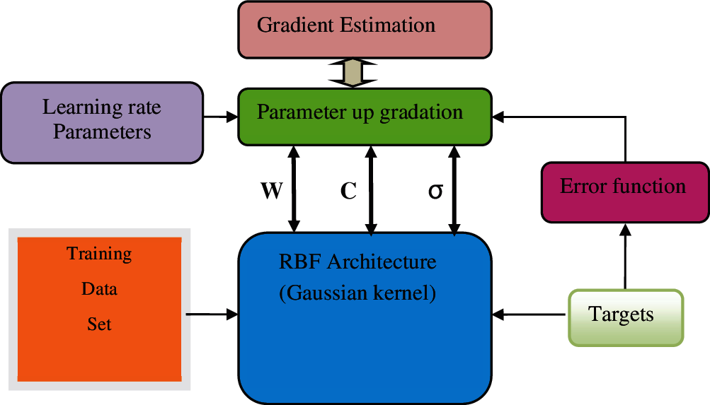
Figure 1: Proposed adaptive RBF working flow

R2=∑(Y^i−Y¯)2∑(Yi−Y¯)2 (10)

where Yi& Y^i are the expected and obtained value correspondingly while Y¯ is the mean value of forecast variable Y. It is the obvious that value of R2 closer to 1 is a better predictor.

4.2 Mapping Based Forecasting

First, consider a forecasting problem from a mapping point of view where for given inputs in one domain to mapped the output in the other domain. The complexity of the problem appears in the forming of the mapping function. The area of application has been considered as the demand for power supply by houses contains various indexes of power consumption like the size of houses, the capacity of air conditioning machines, and the appliance index of the house which included various machines and devices cause of power consumption. The details of the data set have given in Appendix A. Broadly there parameters are good enough to capture a close approximate of the real demand of power consumption by individual houses with this 3 parameters model has to develop to predict the demand of power consumption. To get the details of different possible models by neural network the choice of feed-forward architecture is obvious with supervising learning. Hence, two different architectures, multilayer perceptron-based feed-forward (MLP) and radial basis function neural network have been considered. Gradient-based learning has been applied in both neural models. The size of both networks has been considered as [3, 3, 1] there were uni-polar sigmoid transfer functions in the MLPNN active nodes while Gaussian function in the RBF NN. The learning and momentum rate values were 0.3 in the weight up-gradation of MLPPNN and RBF. Low value ensures smoothness in the learning process which is needed in the appropriate mapping function development. The two different strategies have been applied in model development with RBFNN. First, one, called static RBF (SRBF) where spreads and center of Gaussian function remain fixed with the progress of learning and only output layer weights updated while other models are called adaptive RBF (ARBF), where all the three parameters were updated (as given in section 3). All three network models have given chance to evolved up to 1000 iterations and to mitigate the random variation, 10 independent trials have been given with individual models. The convergence characteristics over 10 independent trials for MLPNN, SRBF, and ARBF have shown in Figs. 2–4. It can observe that there were nearly similar patterns of convergence have been appeared for MLPNN and final convergence has appeared around 400 iterations. With these convergence characteristics, it can be said that MLPNN has shown a high level of stability over different trails and can be reliable.

The convergence for SRBFNN over 10 trials has shown the complexity of learning because of the availability of single parameters (output layer weights) for error minimization. Convergence is very fast but having diversity in nature and heavily depends upon the initialization process of available parameters in the network that is why some convergence was mature while some were immature as shown in Fig. 3. In conclusion, convergence characteristics do not ensure the reliability of outcomes.

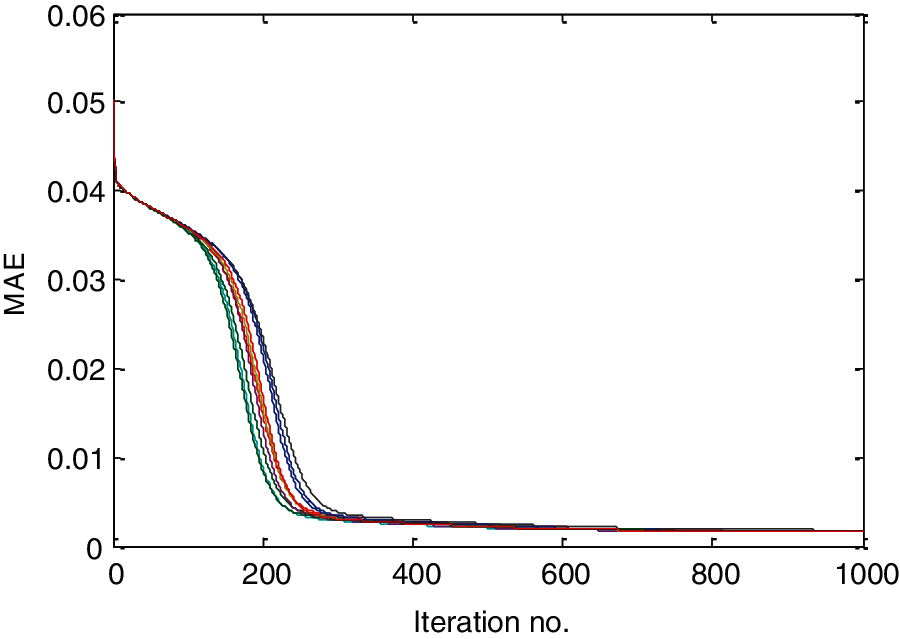
Figure 2: Convergence characteristics of MLPNN over 10 independent trials

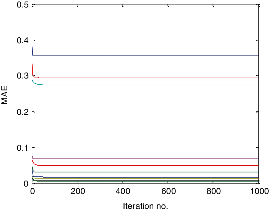
Figure 3: Convergence characteristics of SRBFNN over 10 independent trials

The convergence characteristics of ARBF in Fig. 4 show the benefits of indulging more parameters in the process of learning. For all the trials there was very fast and mature convergence not only that all trials have followed the nearly same path. Hence, the convergence characteristics ensure the faster, global and reliable outcomes from this model. The comparison between all three models from the convergence point of view has shown in Fig. 5, where the mean of all 10 independent trials has been considered. SRBF convergence is poor while the final convergence of MLPNN is nearly the same as ARBF but has taken a long time comparatively. Overall, ARBF has outperformed others. The mean forecast outcomes over the training data and test data by all the three models have shown in Figs. 6 and 8 while the corresponding error in their forecast has shown in Figs. 7 and 9. It can observe that MLPNN and ARBF performance s were very close to expected values while even though SRBF was able to capture the non-linearity but significant differences in predicted values in comparison to the desired one.

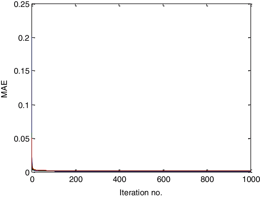
Figure 4: Convergence characteristics of ARBFNN over 10 independent trials

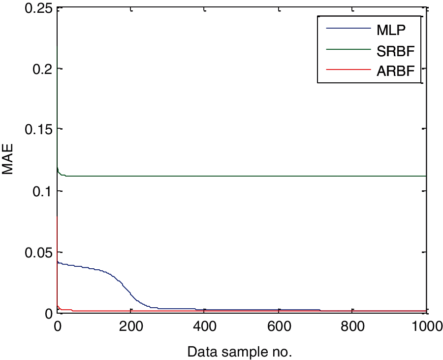
Figure 5: Mean convergence characteristics over 10 independent trials

Over the test data set, performances of ARBF were superior and very close to expected values as shown in Fig. 8. History of under performance in the training phase was repeated by SRBF in the test phase also which was expected as shown in Fig. 9. Predicted outcomes of MLPNN were better than SRBF and closer to ARBF but in comparison to learning phase performance, there was little more error in predicted outcomes as shown in Fig. 9.

The obtained numeric values of standard deviation in the absolute error, mean absolute error (MAE), and estimated R2 values for all the three models over data set for training and test have shown in Tabs. 1 and 3 while to get the crisp comparison their mean performances have shown in Tab. 2. The obtained diversity in the convergence of SRBF as shown in Fig. 3 has affected in terms of their performances as shown in Tab. 1. There was consistency in performances of MLPNN and ARBFNN have been observed as well qualities of prediction were very good. The precise prediction quality performance using R2 have shown in Fig. 10 as a bar plot for all the three models. It can observe that ARBF prediction quality is very near to the ideal predictor (R2 = 1).

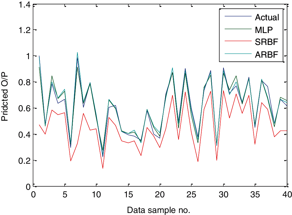
Figure 6: Mean predicted output over training data samples

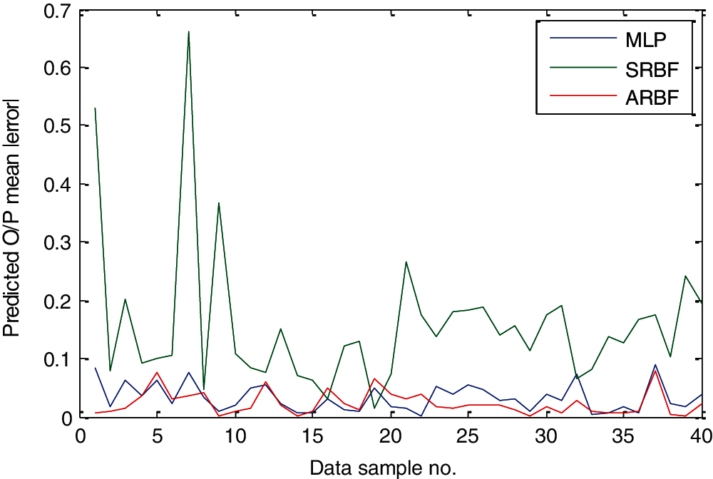
Figure 7: Mean absolute error in prediction over training data

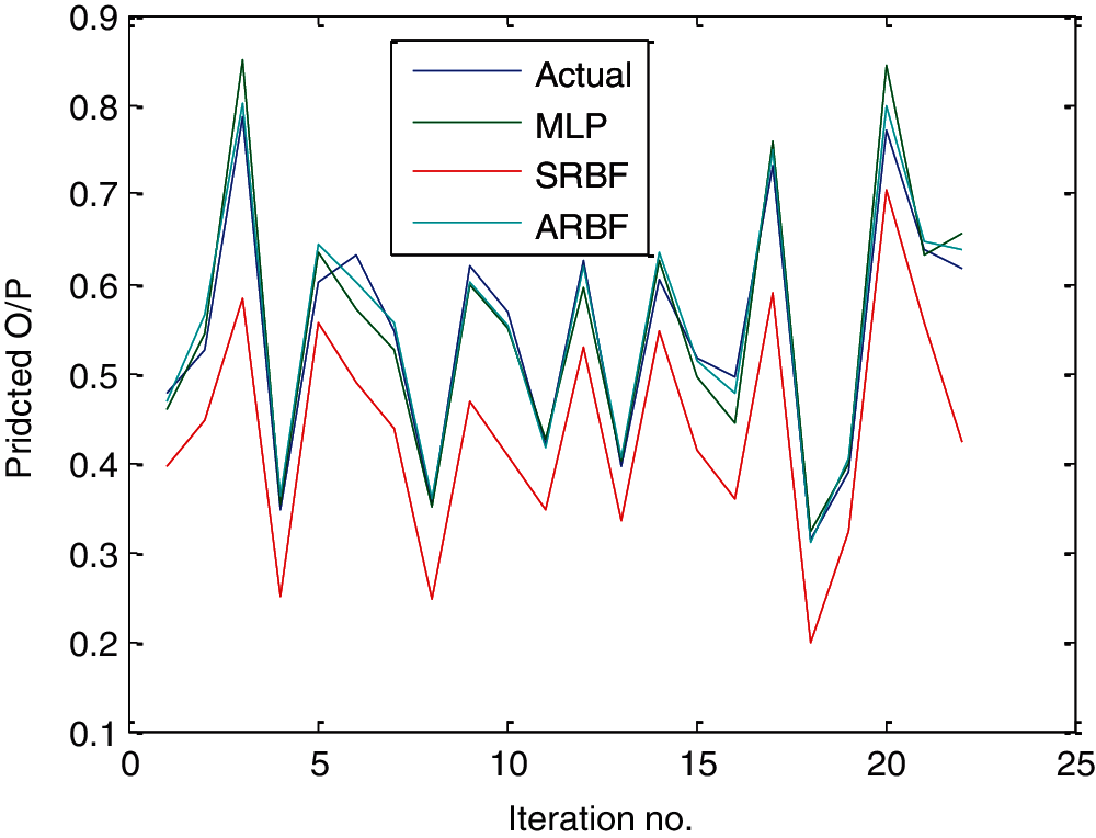
Figure 8: Mean predicted output over test data samples

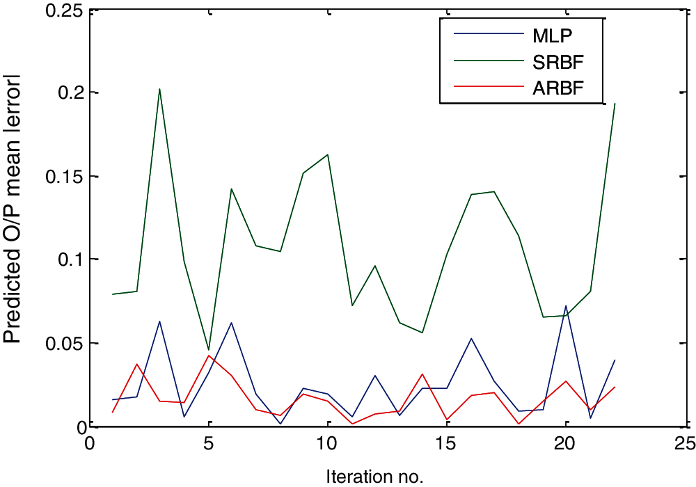
Figure 9: Mean absolute error in prediction over test data samples

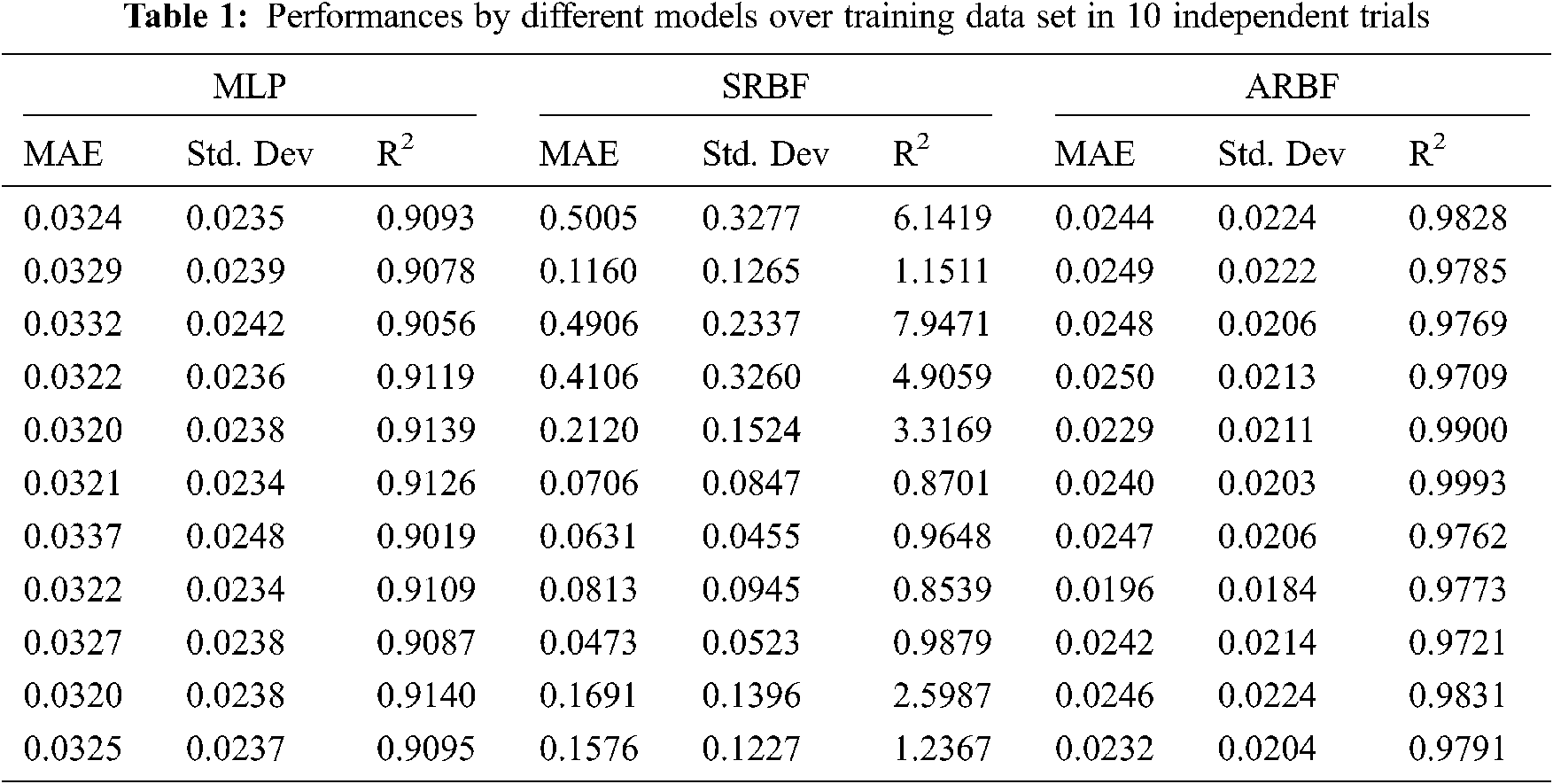
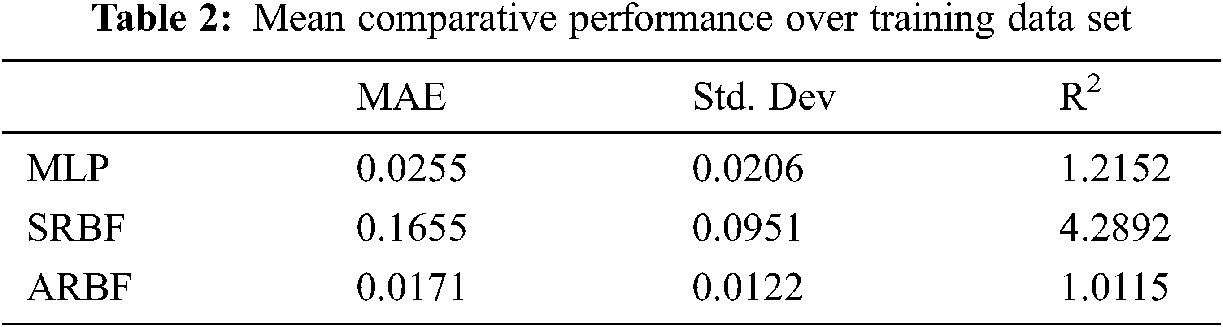
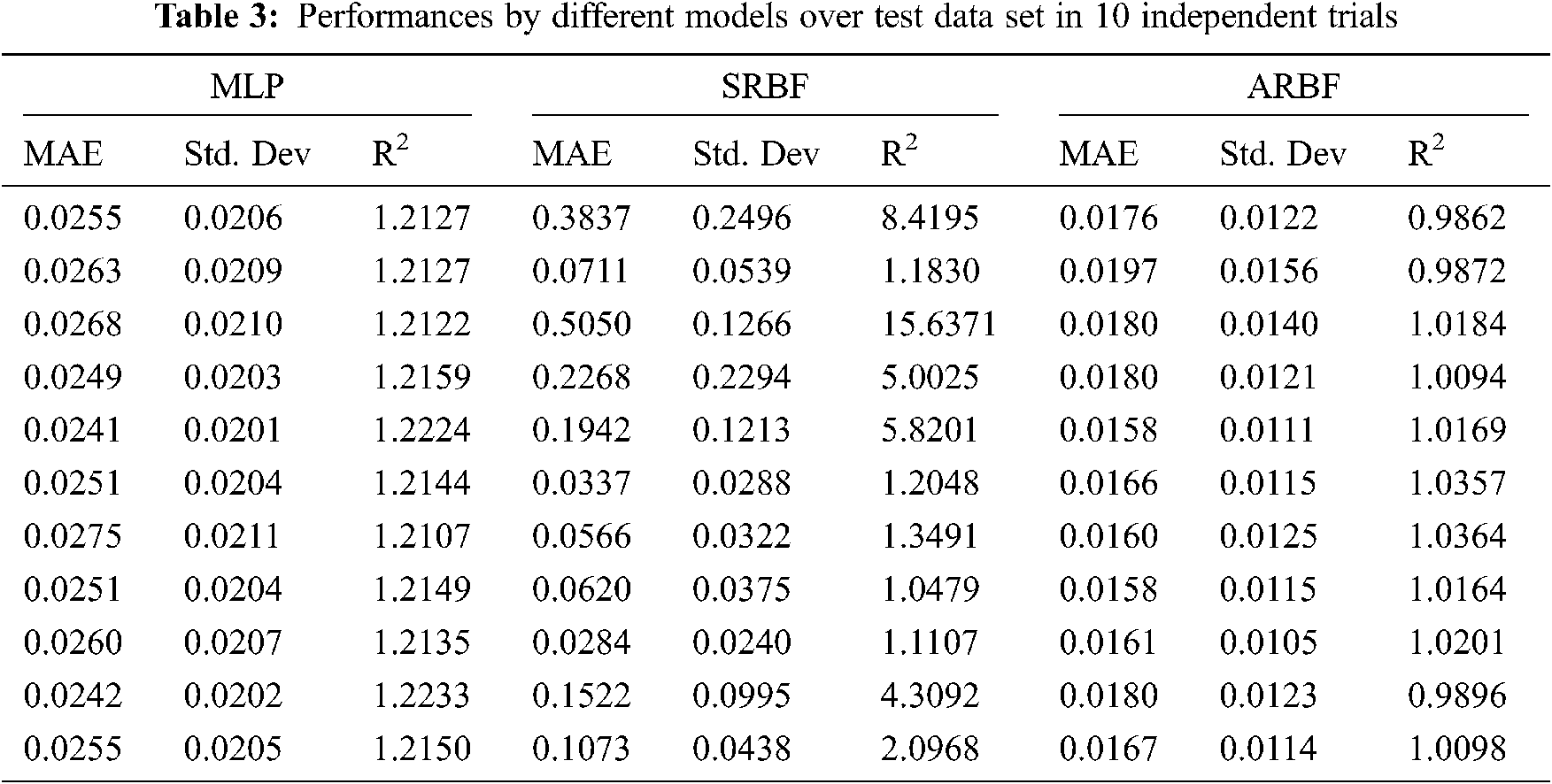
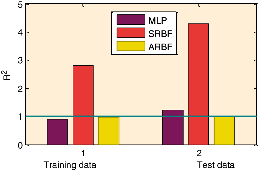
Figure 10: Predicting capability comparison using R2

5  Proposed Hybrid Models for Trend-Cycle Time Series Data Forecasting

The proposed models have been applied in a more complex environment where time-series data (carried the trend and cycle pattern together) have been considered for prediction. To make the prediction more complex there is no immediate relation establishment made by considering the problem of predicting data which are far over a while. Hence there is no benefit of placing the time-lag model where only a next time data sample enters in the input domain in association with previously established correlation by other input samples. In this work, the prediction of net power generation every year by U.S electric companies has been considered for the application and the details have given in Appendix B. The present problem of forecasting has been defined as: “forecast the net power generation month wise for a year from just previous year information”. There were 10 years of data from 1985 to 1995 having the net power generation from the month of January to December every year. Let’s first investigate the characteristic of data as shown in Fig. 11. It can observe that there are two different patterns available in this time series data one is an increasing trend pattern and another one is a cyclic pattern which can be observed by noting the two peaks every year: in mid-summer and mid-winter.

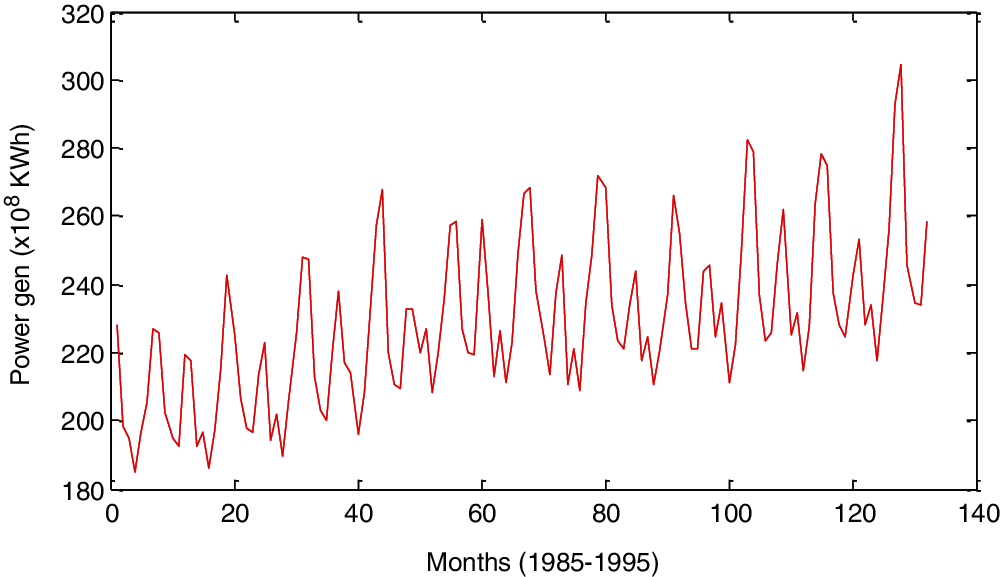
Figure 11: Time series of power generation

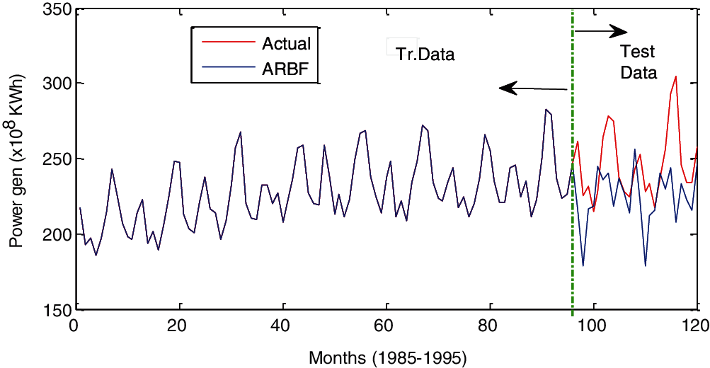
Figure 12: Predicted outcomes by ARBF over training and test data set of power generation

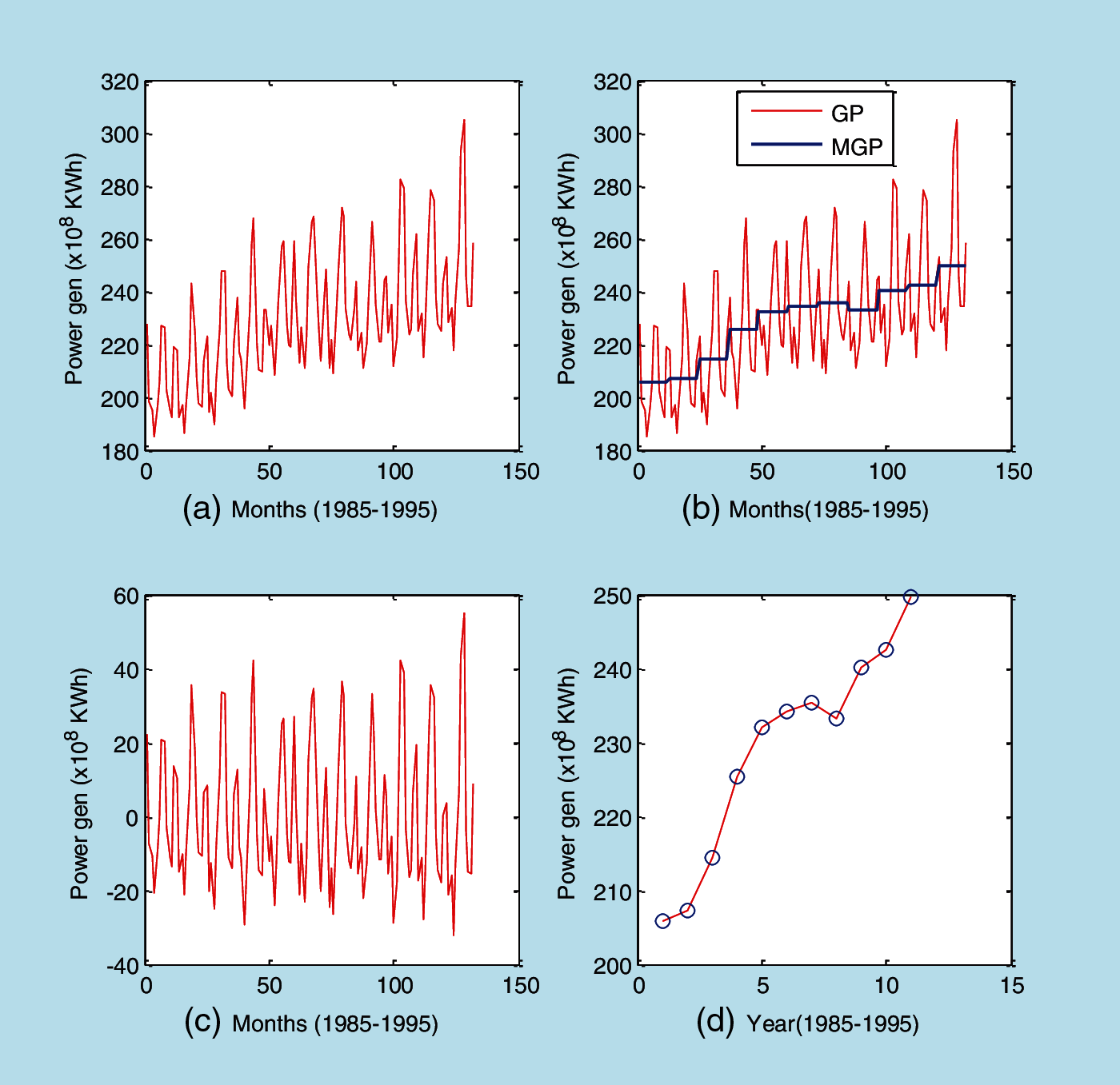
Figure 13: (a) Complete time series data of power generation carried the trend-cyclic pattern (b) Year mean generated power (MGP) in total generated power (GP) (c) Cyclic pattern after removal of mean values (d) increasing trend of year mean power generation year mean power generation

Over this time series data a neural predictor model ARBF, as discussed in Section 3.1, has been developed which has an architecture size of [12, 10, 12] over the training of the first 8 years of data. The predicted performance over the training and test data have shown in Fig. 12. It can observe that ARBF has completely learned the training data but very poor prediction has been observed over test data. This has shown a very serious limitation with the neural network-based predictor model in predicting the mixed pattern time series data.

To overcome this limitation a decomposition method has been proposed which worked in two stages. In the first stage, the trend pattern as observed by considering the mean year power generation as shown in Fig. 13b has been extracted from data and plotted in Fig. 13d to confirm the availability of the increasing trend. The remaining pattern carried the cyclic pattern characteristics as shown in Fig. 13c. For trend patterns, a simple regression model has been applied to predict the next year’s mean power generations from the previous year’s mean value. An ARBFNN predictor model has developed over cyclic pattern data. The function block diagram of the whole process has shown in Figs. 14 and 15.

First, there is the normalization of data which makes the upper limit of data as 1 while positive bias has applied further by adding the positive value to make all value positive only. The same sign of data will make the learning process faster. The same previously considered ARBFNN has been applied to form the cyclic pattern neural predictor. In the test phase, both predictors’ outputs combined. Post-processing is the reverse process of pre-processing and carried the function of the level downshifting and de-normalization. The developed predictor from this process has given a name as DARBFNN which is a hybrid predictor of simple regression and ARBFNN.

The comparative prediction performances by different models over the training data have shown in Fig. 15. It is very interesting to observe that MLNN has failed to capture the monthly variations in power generation and learned to predict the nearly year mean value. SRBF has shown a little better here and learned successfully the monthly variations but for some years there was a large deviation from an actual value. As discussed earlier, ARBF performances were very good over training data and very small errors existed in prediction. The proposed decomposition-based model DARBF has also shown very good performances but a little higher error in prediction in comparison to ARBF as shown in Fig. 16.

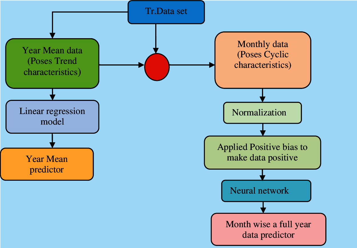
Figure 14: Decomposition based predictor model development for trend-cyclic pattern time series

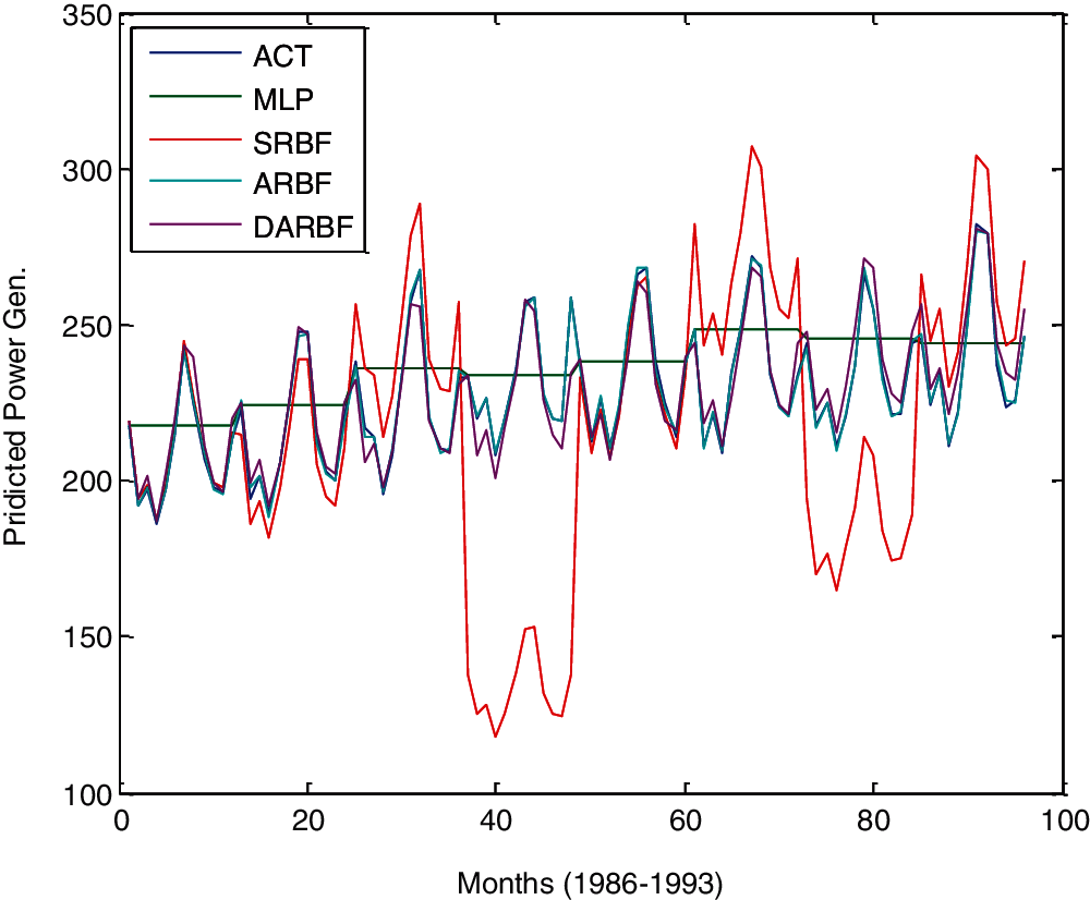
Figure 15: Prediction performances by different models over training data

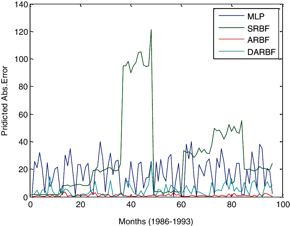
Figure 16: Prediction error by different models over training data

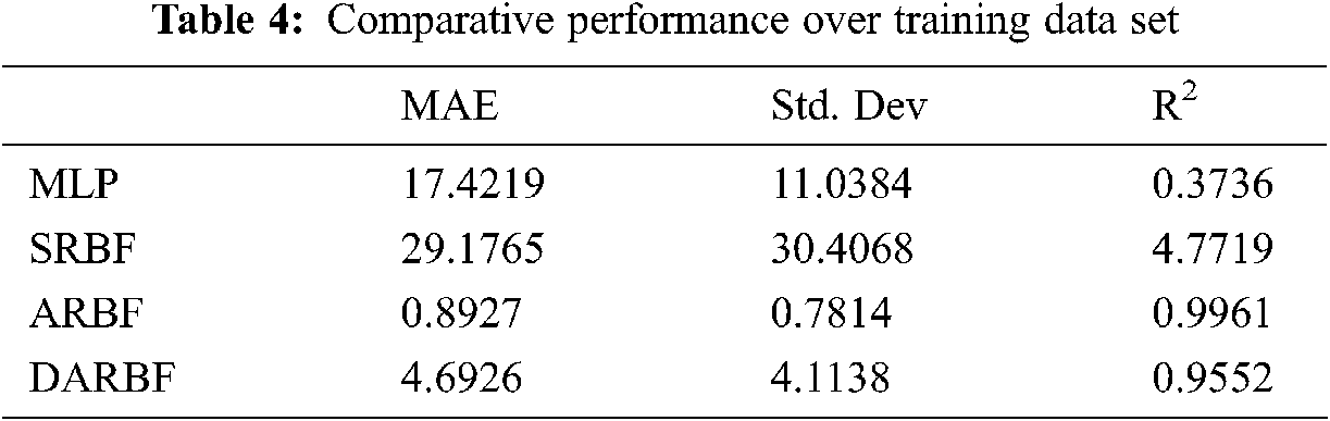
The numeric performance comparisons by different models over the training data and test data have shown in Tabs. 4 and 5. The MLPNN model has shown better performance indexes values in comparison to the SRBFNN model because predicted values were closer to the year mean value. The outcomes of ARBFNN models have significantly improved if it has enclosed under decomposition-based modeling as DARBF.

6  Conclusion

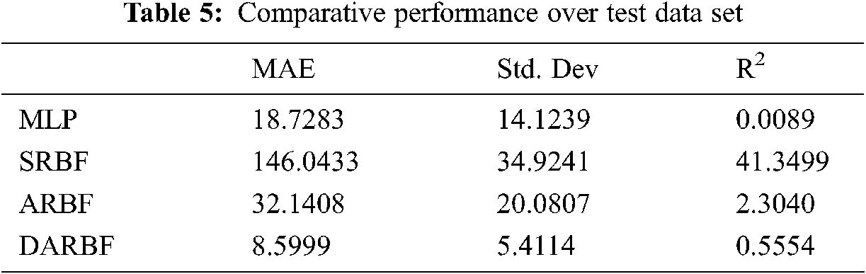
The restriction of static basis function parameters is caused by slow and unsatisfactory learning in the conventional RBF neural network. To overcome this issue adaptive approach has been proposed in the basis function parameters along with weights as result there were three degrees of freedom in error minimization. The prediction based on function mapping was very satisfactory with the use of MLPNN and ARBFNN based predicting models while these models had shown difficulties in prediction of mixed pattern of trend and cyclic in a time series data. The difficulty of the individual predictor has been minimized by the decomposition approach where the component of mixed time series has been separated and the corresponding predictor has been developed. Forecasting application of power demand and power generation has been considered. With the experimental analysis, benefits of ARBF have been confirmed against SRBF or MLPNN in function mapping based forecasting while has been used as a successful component predictor for cyclic pattern prediction in association with linear regression which has been used for increasing trend predictor to predict the outcomes of mix pattern time series. In future work, to develop a better predictor model through linear regression, the coefficients of linear regression can be explored in solution space through computational intelligence to increase the level of accuracy.

Acknowledgement: This research work has been completed in Manuro Tech Research Pvt. Ltd., Bangalore, India, under the program of Innovation with Computational Intelligence (ICI).

Funding Statement: The authors received no specific funding for this study.

Conflicts of Interest: The authors declare that they have no conflicts of interest to report regarding the present study.

This work is licensed under a Creative Commons Attribution 4.0 International License, which permits unrestricted use, distribution, and reproduction in any medium, provided the original work is properly cited.