Intelligent Automation & Soft Computing DOI:10.32604/iasc.2022.022573
Article

Synovial Sarcoma Classification Technique Using Support Vector Machine and Structure Features

P. Arunachalam1, N. Janakiraman1,*, Arun Kumar Sivaraman2, A. Balasundaram3, Rajiv Vincent2, Sita Rani4, Barnali Dey5, A. Muralidhar2 and M. Rajesh2

1Department of Electronics and Communication, K.L.N. College of Engineering, Madurai, 630612, India
2School of Computer Science and Engineering, Vellore Institute of Technology (VIT), Chennai, 600127, India
3School of Computer Science and Engineering, Centre for Cyber Physical Systems, Vellore Institute of Technology (VIT), Chennai, 600127, India
4Department of Computer Science and Engineering, Gulzar Group of Institutions, Khanna, 141401, India
5Department of Information Technology, Sikkim Manipal Institute of Technology, Sikkim Manipal University, Sikkim, 737136, India
*Corresponding Author: N. Janakiraman. Email: janakiraman.n@klnce.edu
Received: 11 August 2021; Accepted: 13 September 2021

Abstract: Digital clinical histopathology technique is used for accurately diagnosing cancer cells and achieving optimal results using Internet of Things (IoT) and blockchain technology. The cell pattern of Synovial Sarcoma (SS) cancer images always appeared as spindle shaped cell (SSC) structures. Identifying the SSC and its prognostic indicator are very crucial problems for computer aided diagnosis, especially in healthcare industry applications. A constructive framework has been proposed for the classification of SSC feature components using Support Vector Machine (SVM) with the assistance of relevant Support Vectors (SVs). This framework used the SS images, and it has been transformed into frequency sub-bands using Discrete Wavelet Transform (DWT). The sub-band wavelet coefficients of SSC and other Structure Features (SF) are extracted using Principle Component Analysis (PCA), Linear Discriminant Analysis (LDA), and Quadratic Discriminant Analysis (QDA) techniques. Here, the maximum and minimum margin between hyperplane values of the kernel parameters are adjusted periodically as a result of storing the SF values of the SVs in the IoT devices. The performance characteristics of internal cross-validation and its statistical properties are evaluated by cross-entropy measures and compared by nonparametric Mann-Whitney U test. The significant differences in classification performance between the techniques are analyzed using the receiver operating characteristics (ROC) curve. The combination of QDA + SVM technique will be required for intelligent cancer diagnosis in the future, and it gives reduced statistic parameter feature set with greater classification accuracy. The IoT network based QDA + SVM classification technique has led to the improvement of SS cancer prognosis in medical industry applications using blockchain technology.

Keywords: Synovial sarcoma; quadratic discriminant analysis; support vector machine; receiver operating characteristics curve; discrete wavelet transform

1  Introduction

Medical industry applications are one of the fastest growing industries in the world for diagnosing diseases with the help of IoT applications through blockchain technology to protect patients from harmful chronic diseases. In which, the modern advances in digital clinical histopathology images have proposed numerous cancer cell classification techniques for brain, breast, cervix, liver, lung, prostate and colon cancer [1–3]. A Synovial Sarcoma (SS) is often occurring commonly in the extremities of adolescents and young adults [4]. It has a variety of morphological patterns, but its chief forms are monophasic and biphasic spindle cell patterns [5]. Histologically, in SS cancer image, the spindle cell patterns seem to be a small oval-shape structure, and it is called as spindle shaped cell (SSC) [6]. The Histopathological Image Analysis (HIA) for cancer classification is impeded by the reasons such as, (1) nonspecific clinical measurements misleading, (2) stained slide preparation, and (3) different medical imaging modalities [7]. The precise classification of normal and abnormal cancer cells is based on the diameter, shape, size, and cytoplasm of features [8]. These features provide the basic and significant information to the pathologists for appropriate treatment plans. Furthermore, the pivotal points of cancer cell classification have been focused in the literature review section.

Over the past three decades, many researchers have examined the problem of identifying which features are useful for differentiating either normal or abnormal cancer cells [9]. Most of the normal cells have a nucleus diameter of 5 to 11 microns, and it is suggested to be almost unchanged. Whereas abnormal cells with a diameter of 18 micron nuclei has been reported to have increased the size of the nucleus in the stained bio-marker region [10]. These above features are normally designated in the name of subjective, local, global, morphological, statistical texture feature set, and Haralick by the classification techniques [11]. Numerous mathematical approaches have been adopted, including linear discriminators, Bayesian classifiers, nearest-neighbor classifiers and more, for cancer cell classification [12].

The cancer classification was performed by kappa statistics in the HIA of biopsy tissue specimens [13]. Due to the limitations in human practice, a computerized system is needed to diagnose cancer, and it can help the pathologist, as well as it is possible to develop an independent system for cancer classification [14]. A cancer nucleus is classified into one of five staining intensity classes (negative, weak, moderate, strong, and very-strong) using Radial Basis Function (RBF) neural networks [15,16]. The drawbacks in this classification have been rectified using Linear Discriminant Analysis (LDA) and k-Nearest Neighbor (k-NN) classifiers [17].

This classification accuracy is improved by fractal analysis including correlation, entropy, and fractal [18]. Grading the histopathological images using energy and entropy features calculation from the multiwavelet coefficients of an image is proposed in [19]. Both the global features (color and texture characteristics of the entire image) and the morphometric features (spatial relationship between histological objects) are concentrated in [20]. The performances of several existing classifiers such as Gaussian, k-NN, and Support Vector Machine (SVM) have been subsequently evaluated. The characteristics of texture feature using the combination of entropy based fractal dimension estimation and Differential Box-Counting (DBC) method has been analyzed in [21]. The Higher Order Statistics (HOS) and spectra based approach provides more valuable information on the variability between cancer and non-cancer cell patterns with respect to different stages and grading [22].

The segmentation of objective features with help of region of interest (ROI) using Boosted Bayesian Multiresolution (BBMR) technique has been proposed by [23]. The statistical texture features set, and Gabor filter are used in Adaboost ensemble method to increase the decision boundary for better classification [24]. The classification of cluster-area in white, pink, and purple color features of colon images have been focused in [25]. Subsequently, the geometric features have been proposed to better quantify the elliptical nature of epithelial cells for the classification of colon images using Hybrid Feature Set (HFS) [26]. The types of training set analysis methods and its corresponding classes of feature extractions using SVM are mentioned in [27]. Spindle Shaped cells (SSC) are specialized cells that are longer than they are wide. They are found both in normal, healthy tissue and in tumors.

In practical situations, unexpected rare tumor is not included in the training data due to different staining (bio-markers) processes. However, in discrimination model, SVMs have also forcibly categorized the above rare tumor into pre-defined classes. Handling of rare tumor is always a complex problem, and it leads to reduce the accuracy of classification between cancer and non-cancer cells [28]. Hence, SVMs seek one-class kernel parameter, and it is determined based on either PCA or LDA. Further, it has been applied to the histopathological images by few researchers so far. According to Tab. 1, most of the researchers have proposed SVM based methods, but they have not yet applied structure based feature components classification particularly in SS cancer images [29,30]. This has paved the way to focus on cancer classification using structure based feature components.

SVM integrated SF and blockchain technologies lead to access to a wide range of histopathological imaging data for processing the cancer classification [31]. Storing and sharing of histopathological imaging data through a decentralized and secure IoT network can lead to in-depth learning in health care centers and medical industry [32]. Here, the input images are decomposed into frequency sub-band coefficients using Discrete Wavelet Transform (DWT). Then the extraction of lower dimensional features set is performed for the distribution of sub-band coefficients using PCA, LDA, and QDA. Those feature sets are considered as inputs to the SVM classifiers. Here, three types of kernel functions are used to classify the cancer and non-cancer cell structure, such as linear, RBF, and Analysis of Variance Randomized Block (ANOVA RB). The rest of this paper is organized as follows. The brief descriptions of basic theories, features components, and SVM formulation are given in Section 2. The classification accuracy of experimental results is analyzed and compared in Section 3. The importance of structure based feature components, SVM classifiers and kernels are discussed in Section 4, and the summary of the analysis is given in Section 5.

2  Materials and Methods

In this section, mathematical definitions of DWT, PCA, LDA, QDA and SVM with three kernel trick functions are intuitively explained.

2.1 Discrete Wavelet Transforms (DWT)

The DWT is a discrete set of wavelet scales and translations with some rules, and it is an implementation of discrete time series known as DWT. The discrete sample function f(n) and the resulting coefficients [33,34] are known and the DWT transform pair of f(n) is defined by

WS(j0,k)=1M∑n⁡f(n)sj0,k(n) (1)

Wψ(j,k)=1M∑n⁡f(n)ψj,k(n) (2)

where j0 is an arbitrary starting scaling, for j ≥ j0 and the DWT of function f ∈ L2(R) related to wavelet function ψ(n) and scaling function s(n) is defined as

Wf(x)=1M∑k⁡Ws(j0,k)sj0,k(n)+1M∑j=j0∞⁡∑k⁡Wψ(j0,k)ψj,k(n) (3)

where sj0,k(n) and ψj,k(n) are the functions of discrete variables and normally j0 = 0, (i.e., M = 2j), n = 0, 1, 2, …, M − 1, j = 0, 1, 2, …, J − 1 and k = 0, 1, 2, …, 2j − 1. These two functions are mathematically expressed by scaling and translation operation using

sj,k(n)=2j/2S(2jn−k) (4)

ψj,k(n)=2j/2ψ(2jn−k) (5)

The standard Haar wavelet and the discretized scaling and wavelet functions are employed corresponding to the Haar transformation matrix of the row M × M which is obtained from Haar basis function, and it is defined as

ψ0(n)=ψ00(n)=1N,n∈[0,1] (6)

and

ψk(n)=ψpq(n)=1N{+2p/2(q−1)/2p≤n<(q−0.5)/2p−2p/2(q−0.5)/2p≤n<q/2p0Otherwise,n∈[0,1] (7)

where, k = 2p + q − 1, 0 ≤ p ≤ n − 1, q = 0 or 1 for p = 0, and 1 ≤ q ≤ 2p for p ≠ 0.

2.2 Principal Component Analysis (PCA)

In PCA, mathematical representation of linear transformation of original image vector into projection feature vector [35] is given by

Y=WTX (8)

where, Y is the m × N feature vector matrix, m is the dimension of feature vector, and transformation matrix W is an n × m, whose columns are the eigenvectors (I) corresponding to the eigenvalues (λ) computed using λI = SI. Here, the total scatter matrix S and the average image of all samples are defined as

S=∑i=1N⁡(xi−μ)(xi−μ)T (9)

where, μ=1N∑i=1N⁡xi . After applying the linear transformation WT, the scatter of the transformed feature vectors {y1, y2…yn} is WTSW. In PCA, the projection W is chosen to maximize the determinant of total scatter matrix of the projected samples, that is

W=argMAXw|WTSW|=[w1,w2,…wm] (10)

where, w1, w2, …wm is the set of n-dimensional eigenvectors of S, and m is corresponding largest eigenvalues of S. In other words, the input vector in n-dimensional space is reduced to a feature vector in m-dimensional subspace. As a result, the dimension of the reduced feature vector m is much less than the dimension of the input image vector n.

2.3 Linear Discriminant Analysis (LDA)

The main goal of the LDA is to discriminate the classes by projecting class samples from p-dimensional space into finely orientated line. For a N-class problem, m = min (N − 1; d) different orientated lines will be involved [36]. For example, we have N-classes, X1, X2, …, XN. Let the ith observation vector from the Xj be xji, where j = 1, 2, …, J and i = 1, 2 … Kj. J is the number of classes and Kj is the number of observations from class j. The co-variance matrix is determined in two ways (1) within-class co-variance matrix CW and (2) between-class co-variance matrix CB. They are given as

Cw=∑j=1N⁡Cj=∑j=1N1Kj∑i=1Kj⁡(xji−μj)(xji−μj)T (11)

CB=∑j=1N⁡Nj(μj−μ)(μj−μ)T (12)

where, μj=1Kj∑i=1Kj⁡xji and μ=1K∑i=0K⁡xi are the mean of class j and global mean, respectively.

The projection of observation space into feature is accomplished through a linear transformation matrix T:

y=TTx (13)

The corresponding within-class covariance matrix C¯W and between-class covariance matrix C¯B in the feature space are given as

C¯W=∑j=1N⁡∑i=0Kj⁡(yji−μ¯j)(yji−μ¯j)T (14)

C¯B=∑j=1N⁡Kj(μ¯j−μ¯)(μ¯j−μ¯)T (15)

where, μ¯j=1Kj∑i=1Kj⁡yji and μ¯=1K∑i=0K⁡y¯i . It is honest to show that:

C¯W=TTSWT (16)

C¯B=TTSBT (17)

The linear discriminant is then defined as a linear function for which the objectives function J(T) is given as

J(T)=|C¯B||C¯W|=|TTCBT||TTCWT| (18)

Here, the value of J(T) is maximum, and it can be shown that the solution of Eq. (17) is that ith column of an optimal transformation matrix T is the generalized eigenvector corresponding to the ith largest eigenvalue of matrix CW−1WSB . To obtain the discriminant profile, the LDA classification score (Lik) for a given class k is calculated by the Eq. (19) and it is considered equivalent to the class covariance matrices:

Lik=(Xi−X¯k)T∑pooled−1⁡(Xi−X¯k)−2logeπk (19)

where, Xi is a measurement vector unknown to a sample I; Xk is the mean measurement vector of class k; Σpooled is a pooled covariance matrix; and πk is the prior probability of class k [36].

2.4 Quadratic Discriminant Analysis (QDA)

The QDA classification score (Qik) is estimated for each class k using the variance-covariance matrix and the additional natural logarithmic term, as defined as follows;

Qik=(Xi−X¯k)T∑k−1⁡(Xi−X¯k)+logk|Σk|−2logeπk (20)

where, logk|Σk| is the nature logarithm of the determinant of the variance-covariance matrix Σk; and Σk is the variance-covariance matrix of class k. The variance-covariance matrix (Σk), the pooled covariance matrix (Σpooled), and the prior probability (πk) are calculated as follows;

Σk=1Nk∑i=1Nk(Xi−X¯k)(Xi−X¯k)T (21)

Σpooled=1N∑k=1KNkΣk (22)

πk=NkN (23)

Here, K is the total number of classes, N is the total number of objects in the training set, and Nk is the number of objects in class k [37].

2.5 The Constructing of Support Vector Machine (SVM)

Let us consider two classes case α1 and α2 and we have a set of training data X = {x1, x2, ….., xN} ⊂ PR. The following rules are labelled by the training data.

yi={+1,xi∈α1,−1,xi∈α2. (24)

In appearance, SVM is a binary classifier, and it can evaluate image data points and assign them to one of two classes. The input observation vectors are projected into higher dimensional feature space F. The function f(x) takes the form

f(x)=(v⋅θ(x))+b (25)

With θ: PR → F and v ∈ F, where (⋅) is denoted by dot product. Mostly, all the preferable data in these two classes satisfy the following constraints.

yj(v⋅θ(xi)+b−1≥0,∀i. (26)

Consider the points θ(xi) in F for which the equality in Eq. (26) holds that these points lie on two hyperplanes, the first one is H1:(v  ⋅ θ(xi)) + b = +1 and the other one is H2:(v  ⋅ θ(xi)) + b = −1. These two hyperplanes are parallel and no training points fall between them. The margin between them is 2/‖v‖. Hence, a pair of hyperplanes with a maximum margin can be found by minimizing ‖v‖2 subject to Eq. (26). This problem can be written as a convex optimization technique

Minimize12‖v‖2 (27)

Subject toyi(v⋅θ(xi)+b−1≥0∀i, (28)

where Eq. (27) is a primal objective function and Eq. (28) is a corresponding constraint. Both can be solved by constructing a Lagrange function. Hence, the positive Lagrange multipliers are taken into consideration ωi; i = 1, 2, …, N, one for each constraint in both equations. The Lagrange function [38] is defined by

Lp=12‖v‖2−∑i=0N⁡ωiyi(v⋅θ(xi)+b)+∑i=1N⁡ωi, (29)

The gradient of Lp must be minimized with respect to both v and b values, and they must vanish. The gradients are given by

∂LP∂vs=vs−∑i=1N⁡ωiyiθ(xis)=0,s=1,2,…,p (30)

∂LP∂b=−∑i=1N⁡ωiyi=0 (31)

where p is the dimension of space F. By combining these conditions and other constraints on primal functions and Lagrange multipliers, we obtain the Karush-Kuhn-Tucker (KKT) condition is obtained and it's given by

∂LP∂vs=vs−∑i=1N⁡ωiyiθ(xis)=0,s=1,2,…,p (32)

∂LP∂b=−∑i=0n⁡ωiyi=0 (33)

yi(v⋅θ(xi)+b−1≥0andωi≥0∀i (34)

ωi(yi(v⋅θ(xi)+b−1)=0∀i (35)

Here, v, b and ω are the variables to be solved. From the KKT Eq. (31), the following is obtained

v=∑i=1N⁡ωiyiθ(xi)∑i=1N⁡ωiyi=0 (36)

Therefore,

f(x)=∑i=0N⁡ωiyi(θ(xi)⋅θ(x))+b=∑i=0N⁡ωiyil(xi,x)+b (37)

where l(xi, x) = (θ(xi) ⋅ θ(xj)) is a kernel function that uses the dot product in the feature space.

In this study, three different kernel functions have been used, and they are calculated as follows:

i) Linear kernel :

l(xi,x)=(xiT.xj) (38)

ii) Gaussian Radial Basis Function (RBF) :

l(xi,x)=exp⁡(−γ‖xi−xj‖2) (39)

iii) Analysis of variance randomized block (ANOVA RB) kernel : z

l(xi,x)=∑k=1n⁡exp(−12γ(xik−xjk)2)d (40)

where l(xi, x) is positive definite for values in RBF kernel case, γ=12σ2 is a spreading factor that controls the width of the kernel function, d is the dimensionality or degree of input space, and σ is a standard division. Substitute Eq. (36) into Eq. (29). This leads to maximization of dual function LD as given by

LD=−12∑i=0N⁡∑j=1N⁡ωiωjyiyjlij+∑i=0N⁡ωi. (41)

Here, the dual function incorporates the constraints, and the dual optimization technique is obtained as defined by

Maximize−12∑i=1N⁡∑j=1N⁡ωiωjyiyjlij+∑i=1N⁡ωi (42)

Subject to∑i=1N⁡ωiyi=0, (43)

Both primal Lp and dual LD constraints are represented with same objective function, but with different constructions. On this, optimization of the primal and dual constraints are a type of convex optimization problem and it can be rectified by using the gird-point search algorithm. Finally, the SVM classifier classifies x by the following classification criteria and it is defined by

x∈Classiiff(i)(x)=maxforallj∈M⁡f(j)(x). (44)

where x an input data vector which is entering the classifier and M-dimensional value vector f(i)(x), i = 1, 2, …, M (one dimension for each class) is generated.

3  Experiment Results

Histopathological Synovial Sarcoma (SS) cancer images have been downloaded from the online link http://www.pathologyoutlines.com/topic/softtissuesynovialsarc.html for training the classifier model. The stained slide SS images are collected from the Kilpauk Medical College and Hospital, Government of Tamilnadu, Chennai, India for external validation purpose. In MATLAB, the multispectral color images are stored individually in red, green, and blue components and the size of each image is 128 × 128 pixels, respectively. The total number of images is 5400, the number of samples per second in each image is 49152, and eight iterations have been considered in each image for computation. Most of the medical image classification methods used the ratio of 70% for training the classifier, 15% for internal validation, and 15% for external validation from the overall dataset. The overall procedure and the implementation flow of SSC classification are represented as a block diagram, Fig. 1. A multiclass kernel machine has been implemented to operate on all groups of features simultaneously and combine them without increasing the number of required classifiers.

Figure 1: Block diagram of overall procedure and its internal operation of SSC structure classification

More interestingly, an SVM has two adjustable parameters that should be optimized for margin maximization and error minimization. One is the determination of spreading factor (γ) in each kernel function and grid-search based optimization technique. The grid search is performed by 256 samples with uniform resolution in log2-space, for example, γ is log2γ ∈ { − 126, − 124, − 122, …, 128}. Second is the linear representation and its corresponding weighting coefficients. It is determined by the Lagrangian multiplier (ωi). The higher weighting coefficient with relevant input vectors is called as SVs. This is done by linear algebra, in which the features of basis vectors are considered as a matrix form with a linear transformation as positive and negative labeled data points.

The statistical testing for the internal cross validation work, the non-parametric test such as Mann Whitney U test has been applied with dependent cross-entropy measures to analyze the matching characteristics of decision-making with respect to null-hypothesis (Ho), and alternate-hypothesis (H1). The cross-entropy measures are used to find the cross-information between the observed and the predicted sample variables. The null-hypothesis represents the sample means of minimum cross-entropy, and it provides valuable information about the well separation of two classes based on the hyperplane. The above-mentioned systematic procedure is applied to PCA + SVM, LDA + SVM, and QDA + SVM for the purpose of spreading factor (γ), cross-entropy and p-value determination.

3.1 PCA + SVM

In PCA, the transformed space, in descending order of accounting variance is orthogonal and the sub-band coefficients are jointly-normally distributed. With the help of principal component regression (PCR), it is capable to find out the best fit of regressor coefficients based on the direction of variations among the other pairs of eigenvalues. The eigenvalues and the eigenvectors are determined from the covariance or correlation matrix. When the PC variance is high, it is easier to extract the coefficients which are linearly correlated with each other. It is very helpful to find different multiple groups of pixels based on its intensity relevant to cancer (SSC) or non-cancer (non -SSC) pixels.

The characteristics of data classification based on its highest 68% PC variance and the corresponding kernel functions are shown in Fig. 2a which has most of the data points are inclined to the first component regressor line. Based on the consistent cell structures in PCR with iterative procedure, it is capable to find the regressor lines and these lines are helpful to extract the hidden feature components for cancer classification. The SVM classification with three different kernel functions is represented in the form of inverse mapping l−1 for convenience Figs. 2b, 3c, 3d.

Figure 2: PCA + SVM classification model. (a) PCI 68% variance, (b) Linear, (c) RBF, (d) ANOVA RB

Figure 3: LDA + SVM classification model. (a) LDA feature components, (b) Linear, (c) RBF, (d) ANOVA RB

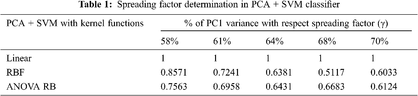
The performance of discrimination between the structured groups of sub-band features depends on the effective prediction of regressor coefficients using the least mean square approach. The null hypothesis of F-statistics is represented in the corresponding feature variables. The spreading factor determination is defined by the proportion of variability in Tab. 1 and that has been explained by the corresponding highest PC. The determination of very narrow spreading factor γ among the data samples is the most important for designing the classifier models perfectly.

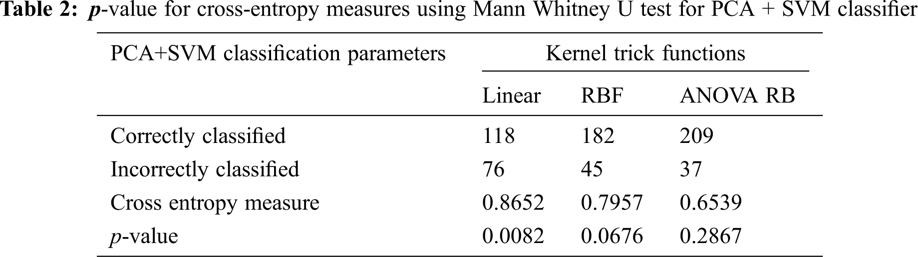
The p-value for accepting the null-hypothesis based on the cross-entropy measures is tabulated in Tab. 2. If the p-value is greater than the significant level (α = 0.05), then the null-hypothesis is accepted. The p-value of 0.0676 is very different to accept the null-hypothesis, even RBF kernel function is used at the same time consistently. It is possible to take the decision to reject the null-hypothesis, when the linear kernel is used. The cross-entropy measure is always less during the transformation using ANOVA RB kernel function, and it provides better performance than other kernels. The ANOVA RB gives better results compared to other two kernel functions and it is a very time-consuming process, when more PCs take influence in PCA.

3.2 LDA + SVM

LDA finds the directions with maximize the variance in between-classes, and minimize the variance in within-classes. The determination of separating the hyperplane between multiple classes is as follows: (1) to find first and second order moments of all classes, (2) to find the individual co-variance matrix for each class, (3) to construct linear equation using mean, standard deviation and co-variance matrix using Eq. (19), and (4) to find the linear line for the separation between two classes using equivalent discriminant function. The major assumption is that identically independently distributed (i.i.d) random variables are represented with either unimodal or multimodal characteristics and its prior probabilities are known in advance. It becomes easier to calculate the between-class Cb and within-class Cw scatter matrices even the cumulative normalized-distance between two classes is very less. It reduces the computation complexity based on relevant discriminant feature extraction.

The dataset and the corresponding discriminator linear line are determined by the identity covariance matrix with a Gaussian distribution of the LDA, as shown in Fig. 3a. The mass of data points is normally distributed towards the middle portion of the scatter plot. The mass of data is separated into two classes using SVM hyperplane, and each of the classes occupies half of the space. The best boundary discrimination is done by example of linear, RBF, and ANOVA RB kernels as shown in Figs. 3b–3d respectively. The boundary is determined by the Bayes rule using the true (normal) distribution.

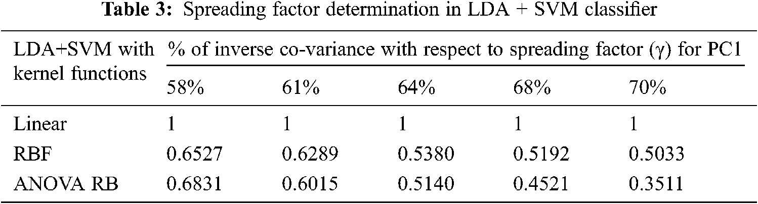
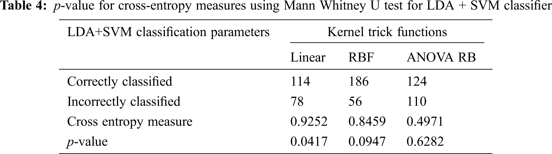
The determination of spreading factor in LDA + SVM with different kernel functions and cross-entropy measures are given in the Tabs. 3 and 4. The average spreading factor is 0.5684 for RBF kernel and 0.52014 for ANOVA RB kernel, when the variance of inverse covariance matrix varies from 58% to 70%. In linear kernel, an alternate-hypothesis is accepted, due to the insignificance p-value during Mann Whitney U test. The spreading factor γ is always unity in linear kernel, and much significance is not possible to attain. The good indication is that the cross-entropy is less than 0.5 in ANOVA RB kernel function. Hence, the performance of LDA depends only on the exact determination of mean and variance of the individual group pixels. The resulting boundaries are well separated between the SSC (∇ plus) over the non-SSC (*) and the best boundary line is improved in ANOVA RB. The discrimination of class Lik gives successive separation between two class feature vectors. Here, it is imperative to increase the performance of linear discrimination.

3.3 QDA+SVM

More Gaussian mixtures of feature components are added to provide the information on each class density by single multivariate Gaussian density function. The covariance matrix of each class is equal to the sum of the data points of all classes. Furthermore, the probability of each class πk is determined at the given data point of k classes and the total number of comparisons is  k−1 . The variance-covariance matrix of the cell structure must have a multivariate normal distribution. Fig. 4a clearly shows two different quadratic discriminant lines which are needed to differentiate the cell structures. The exact classification of kernel functions is shown in Figs. 4b–4d. The individual class probability (πk) takes major contribution to find the best discriminator boundary line. It requires more observations per class (ni >p) ∀ i . The variance-covariance matrix is estimated separately for each class, whereas LDA uses a pooled estimation of a common variance-covariance matrix.

Figure 4: QDA + SVM classification model. (a) QDA feature components, (b) Linear, (c) RBF, (d) ANOVA RB

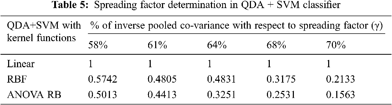
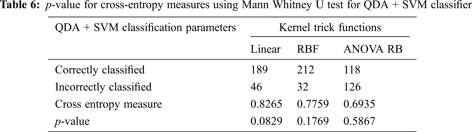
The determination of spreading factor in terms of inverse pooled co-variance matrix is represented in Tab. 5. Due to the less percentage of pooled covariance matrices and the narrowed γ value, all the kernel trick functions are performed well and it has been given in Tab. 6. The mean value of spreading factor is minimum, even the variance of pooled covariance matrix has been increased from 58% to 70%. The transformed data sample using ANOVA RB function does not affect the performance of cross-entropy measure and it always leads to minimum values. Hence, the technique is very good option compared to other two discriminator models for classification.

3.4 Classifiers Evaluation Using ROC

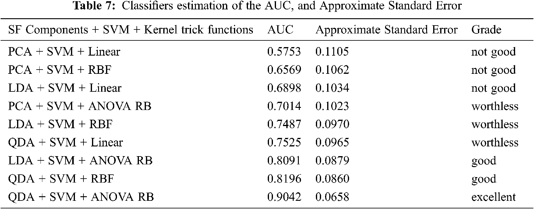
The purpose of external validation is mainly to evaluate the classification performance between the concern feature extraction methods and the kernel functions by ROC curve [38,39]. It is a curve which depicts the interaction between the x coordinate as a 1- specificity and the y coordinate as a sensitivity. These two parameters are mathematically expressed as sensitivity  =  TP/(FN + TP) and specificity  =  TN/(FP + TN) using the confusion matrix. The threshold for the best cut-off range is in-between 0 to 1 with 0.05 uniform interval and 20 samples per parameter. The most common quantitative index for describing the accuracy is expressed by the area under the ROC curve (AUC). It provides a useful parameter for estimating and comparing the classifier performance. The AUC can be determined by Eq. (45). The AUC performance results with different kernel functions are summarized in Tab. 7.

AUC=∑iN−1⁡((1−specificity)i+1−(1−specificityi)∗(sensitivityi+sensitivityi+1))/2 (45)

The grade system of AUC is categorized into four groups, which are excellent, good, worthless and not good, and their common range values are 0.9  < AUC < 1.0, 0.8 < AUC < 0.9, 0.7 < AUC < 0.8 and 0.6 < AUC < 0.7, respectively. Hence, Fig. 5a shows the result of AUC values for PCA + SVM with Linear, RBF, and ANOVA RB kernel functions, and they have an AUC of 0.5753, 0.6569, and 0.7014, respectively. Similarly, LDA + SVM and QDA + SVM with their three different functions, and the ROC curves are shown in Figs. 5b and 5c. The results of AUC values are 0.6898, 0.7487, 0.8091 and 0.7525, 0.8196, 0.9042, respectively. Depending on the AUC value, the QDA + SVM with the ANOVA RB has achieved as the excellent classification model, whereas the LDA + SVM with ANOVA RB and the QDA + SVM with the RBF are good models. Based on these results, it is demonstrated that QDA + SVM with ANOVA RB has been chosen to be applied in the proposed SSC structure classification, because this classifier QDA + SVM with ANOVA RB model has the greatest AUC than the others.

Figure 5: ROC curves of PCA + SVM, LDA + SVM and QDA + SVM classifier models (a) PCA + SVM classifier model (b) LDA + SVM classifier model (c) QDA + SVM classifier model

This ANOVA RB kernel is consistent (Tab. 7), and it possesses the lowest classification error to build a hyperplane model. There is an attractive difference between the two analyses, that is, the classification error and the ROC curve against the occurrence of other two kernels. As a result of approximate standard error, the RBF kernel is better than the linear kernel. With respect to ROC curve analysis, it is clear that ANOVA RB is better than RBF kernel. However, it is stated that the ROC curve analysis is particularly useful for the performance evaluation in the current framework, because it has widely reported that it reflects the true state of a classification problem rather than a measurement of classification error.

4  Discussion

A new approach has been proposed and the SSC structure feature components are extracted and statistically classified using the combination of SVM with different kernel trick functions. When differentiating cancer and non-cancer cells in SS images, the third-level decomposed cell SF is discriminated using PCA, LDA, and QDA techniques, and the nonlinear features are transformed into linear using kernel functions. The direction of variance and its different characteristics of the structured cell pixels are key parameters for the classification. It depends on the input data variables subject to centering. The PCA technique finds the direction of variance among the feature coefficients, but in QDA and LDA, the variances of within-classes and between-classes are considered respectively. Here, LDA uses a pooled covariance matrix and QDA uses each group's variance-covariance matrix. Both techniques are tried to maximize the between-class variability, and minimize the within-class variability based on a Mahalanobis distance calculation.

The kernel trick functions are used to discover the ‘right set of features’ when the mapping function l is non-trivial. The performance analysis is compared based on the transformation of feature coefficients using, (1) Inner product between f(x) and f(x2), (2) Exponential operation with single spreading parameter, and (3) Sum of exponential operation with multiple spreading parameters into the higher dimensionality of the input space. Then, SVM automatically discovers the optimal separating hyperplane in the complex decision surface during mapping back into input space via l−1. The overall comparison performance between SF techniques and kernel trick functions are given in Tab. 8.

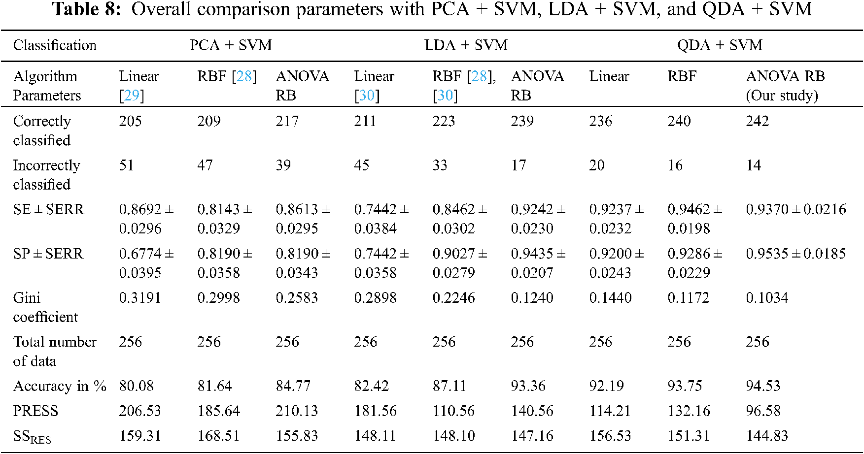
The Gini coefficient is an elementary parameter that measures the superior performance between the classifiers. It is based on the area dominated by the ROC surfaces. The determination of Gini coefficient from the ROC curve is given by Eq. (46).

G=1−∑k=1n⁡((1−specificity)k−(1−specificity)k−1)∗(sensitivityk+sensitivityk−1) (46)

The proposed classification models showed the robustness of classifying SS cancer effectively and accurately in QDA + SVM with ANOVA RB kernel function. The prediction residual error sum of squares (PRESS) statistics shows that QDA + SVM is lower than the sum of square residuals (SSRES) and its average variations of PCA + SVM, LDA + SVM, and QDA + SVM. The main purpose of PRESS statistics is to measure how well the proposed classifier models will perform in predicting the new data. The standard error (SERR) is also specified in each parameter to understand the maximum and minimum variations in sensitivity (SE) and specificity (SP). The QDA + SVM have obtained a higher classification rate than the other classifier models.

ANOVA RB kernel trick function requires less computational time over other kernels functions. This can be used to increase the accuracy of classification, reduce the timing of diagnostic procedures, to speed up treatment plans, and improve prognosis and patient survival rates. This is an opportunity to improve the results with deep learning techniques.

5  Conclusion

The SSC structure classification has been proposed as a new approach and it is totally based on the combination of PCA + SVM, LDA + SVM, and QDA + SVM, for the prediction of relevant structured SVs with the help of kernel trick functions. Based on the experiments carried out in this study, following three conclusions have been drawn such as, (1) QDA based technique does not affect the ‘dependence-observer’ and ‘intra-inter observer’ variability, since there is no general assumption about any practical feature vector datasets, (2) QDA + SVM always trying to maximize the between-class variability while minimizing within class variability based on a distance calculation, and (3) The significant differences in SF component between shape and similarity are studied especially in ANOVA RB kernel trick function. The evidence for structured support vectors and its randomized block variance of a related trick function as few parameters are enough for easier recognition of cancer and non-cancer cells in SS cancer images. In the future, deep learning investigation about SVM can be examined. Therefore, recent support vectors and different structural features will enable future works to achieve integrated blockchain technology based SS image data classification barriers and medical device industrial applications.

Acknowledgement: Our heartfelt thanks to Dr. S.Y. Jegannathan, M.D (Pathologist), DPH, Deputy Director of Medical Education, Directorate of Medical Education, Kilpauk, Chennai, Tamil Nadu, India, who provided valuable advice and oversight in guiding our work.

Funding Statement: The authors received no specific funding for this study.

Conflicts of Interest: The authors declare that they have no conflicts of interest to report regarding the present study.

This work is licensed under a Creative Commons Attribution 4.0 International License, which permits unrestricted use, distribution, and reproduction in any medium, provided the original work is properly cited.