DOI:10.32604/iasc.2022.022643
| Intelligent Automation & Soft Computing DOI:10.32604/iasc.2022.022643 | |
| Article |
Modeling of Anthrax Disease via Efficient Computing Techniques
1Department of Mathematics, Govt. Maulana Zafar Ali Khan Graduate College Wazirabad, 52000, Punjab Higher Education Department (PHED), Lahore, 54000, Pakistan
2Department of Mathematics, National College of Business Administration and Economics, Lahore, 54660, Pakistan
3Department of Mathematics, Cankaya University, Ankara, 06530, Turkey
4Department of Medical Research, China Medical University, Taichung, 40402, Taiwan
5Department of Mathematics, Faculty of Sciences, University of Central Punjab, Lahore, 54000, Pakistan
*Corresponding Author: Muhammad Rafiq. Email: m.rafiq@ucp.edu.pk
Received: 13 August 2021; Accepted: 14 September 2021
Abstract: Computer methods have a significant role in the scientific literature. Nowadays, development in computational methods for solving highly complex and nonlinear systems is a hot issue in different disciplines like engineering, physics, biology, and many more. Anthrax is primarily a zoonotic disease in herbivores caused by a bacterium called Bacillus anthracis. Humans generally acquire the disease directly or indirectly from infected animals, or through occupational exposure to infected or contaminated animal products. The outbreak of human anthrax is reported in the Eastern Mediterranean regions like Pakistan, Iran, Iraq, Afghanistan, Morocco, and Sudan. Almost ninety-five percent chances are the transmission of the bacteria from forming spores by the World Health Organization (WHO). The modeling of an anthrax disease is based on the four compartments along with two humans (susceptible and infected) and others are dead bodies and sporing agents. The mathematical analysis is studied along with the fundamental properties of deterministic modeling. The stability of the model along with equilibria is studied rigorously. The authentication of analytical results is examined through well-known computer methods like Euler, Runge Kutta, and Non-standard finite difference (NSFD) along with the feasible properties (positivity, boundedness, and dynamical consistency) of the model. In the end, comparison analysis of algorithms shows the effectiveness of the methods.
Keywords: Anthrax disease; deterministic modeling; stability analysis; computer methods
The major cause of many diseases in the world is viruses and bacteria. Anthrax is a bacterial disease. Anthrax is a disease of herbivores such as sheep, goats, horses, cows and transmitted to humans. Infected Animals are the source to transmit the bacteria in humans. It does not spread from animal to animal or man to man like covid 19. Anthrax spores can enter the human body through via breathing and cuts on the skin. Its incubation period varies from one to several days. Insects are also the source of the transmission of anthrax. Bacteria are prokaryotes that contain a cell wall, capsule, ribosomes, pili, flagella, and DNA. This species of a bacterium can survive in a harsh environment. Bacteria are considered the eldest living organisms on the earth. The Greek word anthrax means coal. Egypt is the region of anthrax disease. Pieces of evidence show that many scholars of Greece and Rome are well known about anthrax. Anthrax disease is the cause of the downfall of Rome. Those animals which become the victims of anthrax do not show any proper symptoms. They die after infection without leaving diagnostics symptoms. Three forms of anthrax are cutaneous, inhalation, and gastrointestinal. Cutaneous anthrax is about 95% in society. It is a very less dangerous form of anthrax. This form of anthrax usually shows its symptoms for 1 to 7 days. A person can get cutaneous anthrax through cuts on the skin. The persons who are working in tanning and woolen industries can easily get cutaneous anthrax. This form of anthrax is most common in the hands, foot, and neck regions. The common symptoms of cutaneous anthrax are small blisters appear on the skin, looks like an insect bite, swelling in tissues around the sore, a black-centered painless sore appears on the skin such as on the face, hands, and neck regions. We can easily survive by using proper antibiotics. Inhalation anthrax is the most dangerous form of anthrax. It usually shows its symptoms within a week and can become chronic. Its symptoms are fever, feeling cold disorder in the chest, shortness of breath, coughing, vomiting, headache, pain in the stomach, and fatigue. No evidence in the world shows its propagation with infected milk. There is a disorder in the elementary canal on ingesting. sixty percent of patients can easily survive on the proper treatment of gastrointestinal anthrax. The death ratio of humans via anthrax is 20% (cutaneous), 75% (gastrointestinal), and 80% (lung infection). This disease is common in developing countries like the Sahara Desert in Africa, central and southwestern Asia (Turkey, Labnan, Syria, Iran, Egypt), and the Caribbean (Belarus Hungry, Romania, Slovakia). Dozens of cows are died due to anthrax in Pakistan. Mackey et al. studied a model in which describes the transmission of disease in zebras [1]. Baloba et al. investigated the control measures or mechanisms to overcome anthrax [2]. Stella et al. suggested the SIR model for anthrax disease in the animal community [3]. Rezapour et al. proposed a mathematical model for explaining the spread of anthrax with the help of the Caputo-Fabrizio technique [4]. Croicu suggested the IACN model of anthrax disease in herbivores [5]. Gomez et al. suggested the SIML model for transmission of anthrax [6]. Mushayabasa et al. proposed the SEIPC model with the well-known assumptions of mathematics to dispose of carcasses [7]. Roy et al. suggested the SIAC model for the spread of anthrax in animal populations [8]. Mushayabasa suggested the model and its reproduction number with the help of the Lyapunov method [9]. Wanying et al. suggested different factors for controlling the death rate during the bioterrorist attack of anthrax [10]. Pantha et al. studied optimal control of a mathematical model for the spread of anthrax [11]. Gutting studied the inhalation of anthrax in rabbits [12]. Toth et al. estimate the incubation period for the treatment of inhalation anthrax in humans [13]. Day et al. present a model for control of inhalation anthrax [14]. Wilkening proposed an incubation period and describe the importance of the incubation period for controlling inhalation anthrax [15]. Li et al. studied a dynamical mathematical model for the analysis of anthrax disease [16]. Pittman described the importance of the anthrax vaccine in humans [17]. Furniss et al. suggested a model for the control of anthrax in Kruger national park [18]. Pauline described the significance of modeling diseases [19]. Helikumi et al. described the importance of reproduction numbers in modeling various diseases like anthrax [20]. Webb proposed the risk of anthrax in biowarfare [21]. Afshar et al. discussed the detail of a clinical case of anthrax in Iran [22]. Hashemi et al. argued the gastrointestinal patient of anthrax in northeast Iran [23]. Osman et al. developed a model for Listerriosis and anthrax [24]. Brookmeyer et al. suggested the incubation period of anthrax, and they also discussed the incubation period depends on the age and amount of spore that enters in lungs [25]. Karginov et al. discussed that ciprofloxacin with antibodies and the growth of bacteria should be efficient for curing anthrax [26]. Loving et al. described that mice species were more efficient for the study of anthrax [27]. Radosavljevic et al. suggested the curing techniques for the bioterrorist attack of anthrax [28]. Mathematical techniques were studied to analyze the transmission of infectious diseases [29–42]. In this paper, we study the dynamics of anthrax disease via computational methods. We can observe that computational methods in literature have many problems like negativity, unboundedness, and inconsistency of solutions. These issues will resolve by our proposed idea that is a non-standard finite difference method (NSFD). Also, NSFD fulfills the properties of the biological problem. The rest of the paper is styled as follows: In Section 2 the modeling of anthrax is defined. In Section 3 the construction way of the anthrax epidemic model, equilibrium points and computer methods and their convergence are explained. In the last section conclusion and future problems are discussed.
By using the theory of population dynamics of epidemiological type, susceptible and infected is the sum of the total population. The evolution process of the bacteria describes the effect of the epidemiological parameters based on the system of nonlinear coupled ordinary differential equations. Thus, a continuous model for populations regarding anthrax is described in Fig. 1.
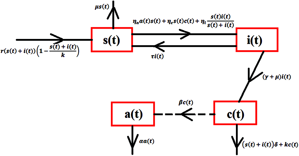
Figure 1: Transmission map of anthrax
The vertical transmission of humans, birth and death rates of humans are considered approximately equal. The physical relationship of variables and constants are shown in Tab. 1 as follows:

The system of differential equations can be deriving from the above flow chart of population as follows:
The system (1-4) is based on the feasible region of the model as follows:
Lemma 1: The solutions
Proof. In this section, we prove the positivity of the first two compartments due to human populations. Forgiven an initial condition
From Eq. (1),
From Eq. (2),
Hence, the system (1-4) admits a positive solution.
Lemma 2: The solutions
Proof. Consider the population function as follows:
Hence, the system (1-4) admits bounded solution and lie in the feasible region
Considering the system (1-4) in which state variables treated as constant and the change in variables are assumed to be zero as follows:
The system (5-8), admitted two types of equilibria that are anthrax free equilibrium (AFE) and anthrax existing equilibrium (AEE). The anthrax existing equilibrium (AEE) is denoted by
where
And the anthrax free equilibrium (AFE) is denoted by
The reproduction number has a significant role in disease dynamics. It presented the ratio of infectivity in the population. For the sake, in the system of anthrax disease, there is only a single compartment is related to infected ness. Without loss of generality, we consider
By assuming the anthrax free equilibrium
Note that,
In this section, we discussed two well-known theorems for stability. Considering the system (5-8) as functions of the equations.
The partial derivatives along with the states variables as follows:
where
The general form of the Jacobin matrix is defined as
Theorem 1: If
Proof. The Jacobean matrix of Eq. (9) at
where
Where
By using the Routh Hurwitz criterion of 3rd order, the following constraint is satisfied
Theorem 2: If
Proof: The Jacobean matrix Eq. (9) at
where
where
where
By using Routh Hurwitz criteria of order 4th, all constraints have been satisfied. So, anthrax existing equilibrium
In this section, we discussed some well-known computer methods like Euler, Runge Kutta, and the non-standard finite difference method for the system (1-4).
This method could be applied in the system (1-4) as follows:
where n = 0,1,2,3… and discretization gap is denoted by h.
This method could be applied in the system (1-4) as follows:
Stage 1
Stage 2
Stage 3
Stage 4
Final stage
where h is any discretization and
3.3 Non-Standard Finite Difference Method
This method could be applied in the system (1-4) as follows:
where h is any discretization and
Theorem 3: For any
Proof. Consider the right-hand sides of the system (15-18), as function W, X, Y, and Z as follows:
The partial derivatives with respect to the state variables as follows:
where
The Jacobean matrix at anthrax free equilibrium is as follows:
where
where
By using the Mathematica, this is guarantee to the fact that all values of Jacobian lie in a unit circle, as desired.
In this section, we used the scientific literature presented in Tab. 2, for the simulating behavior of the system (5-8) at both equilibria of the model as follows:

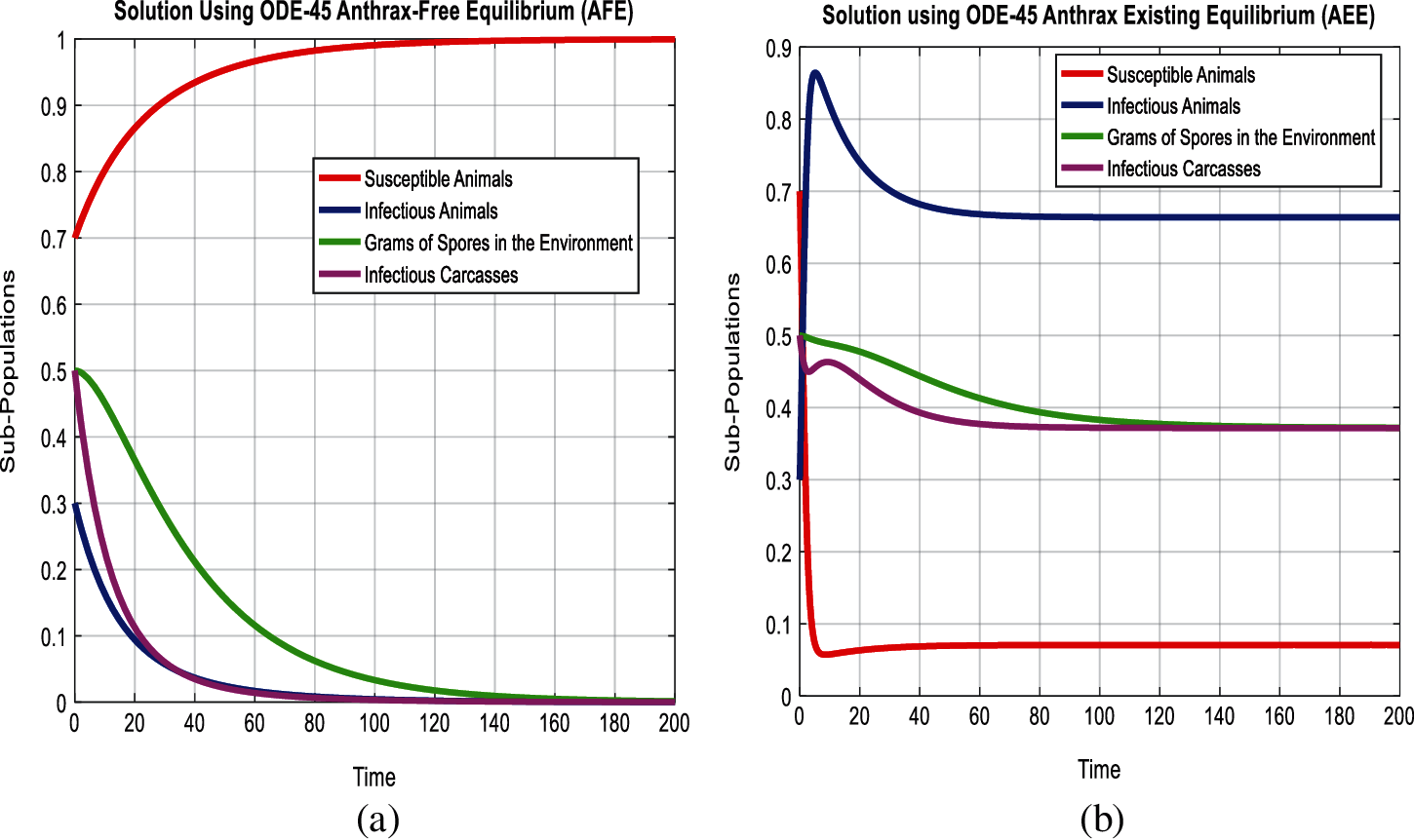
Figure 2: Combined graphical behavior for the equilibria and converges at any time t (a) sub-populations at anthrax-free equilibrium (b) Sub-populations at anthrax existing equilibrium
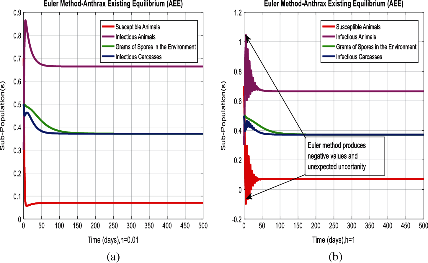
Figure 3: Combined graphical behavior for the equilibria of the model (a) Euler method for sub-populations at anthrax existing equilibrium when h = 0.01 (b) Euler method for sub-populations at anthrax existing equilibrium when h = 1
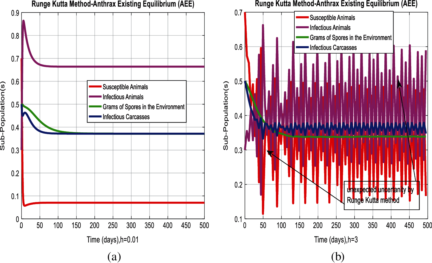
Figure 4: Combined graphical behavior for the equilibria of the model (a) Runge Kutta method for sub-populations at anthrax existing equilibrium when h = 0.01 (b) Runge Kutta method for sub-populations at anthrax existing equilibrium when h = 3
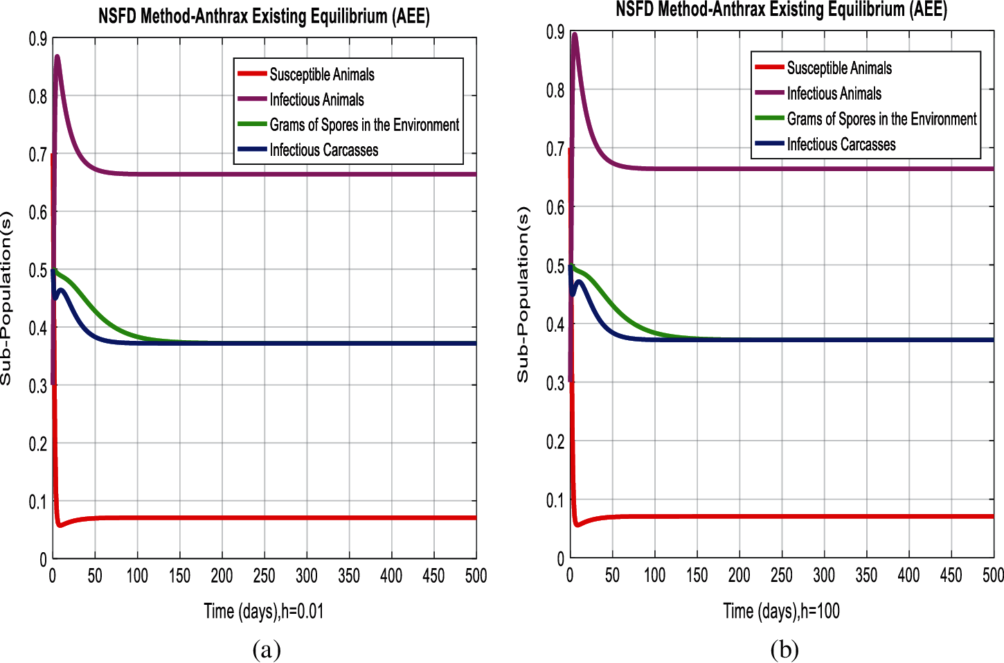
Figure 5: Combined graphical behavior for the equilibria of the model (a) NSFD method for sub-populations at anthrax existing equilibrium when h = 0.01 (b) NSFD method for sub-populations at anthrax existing equilibrium when h = 100
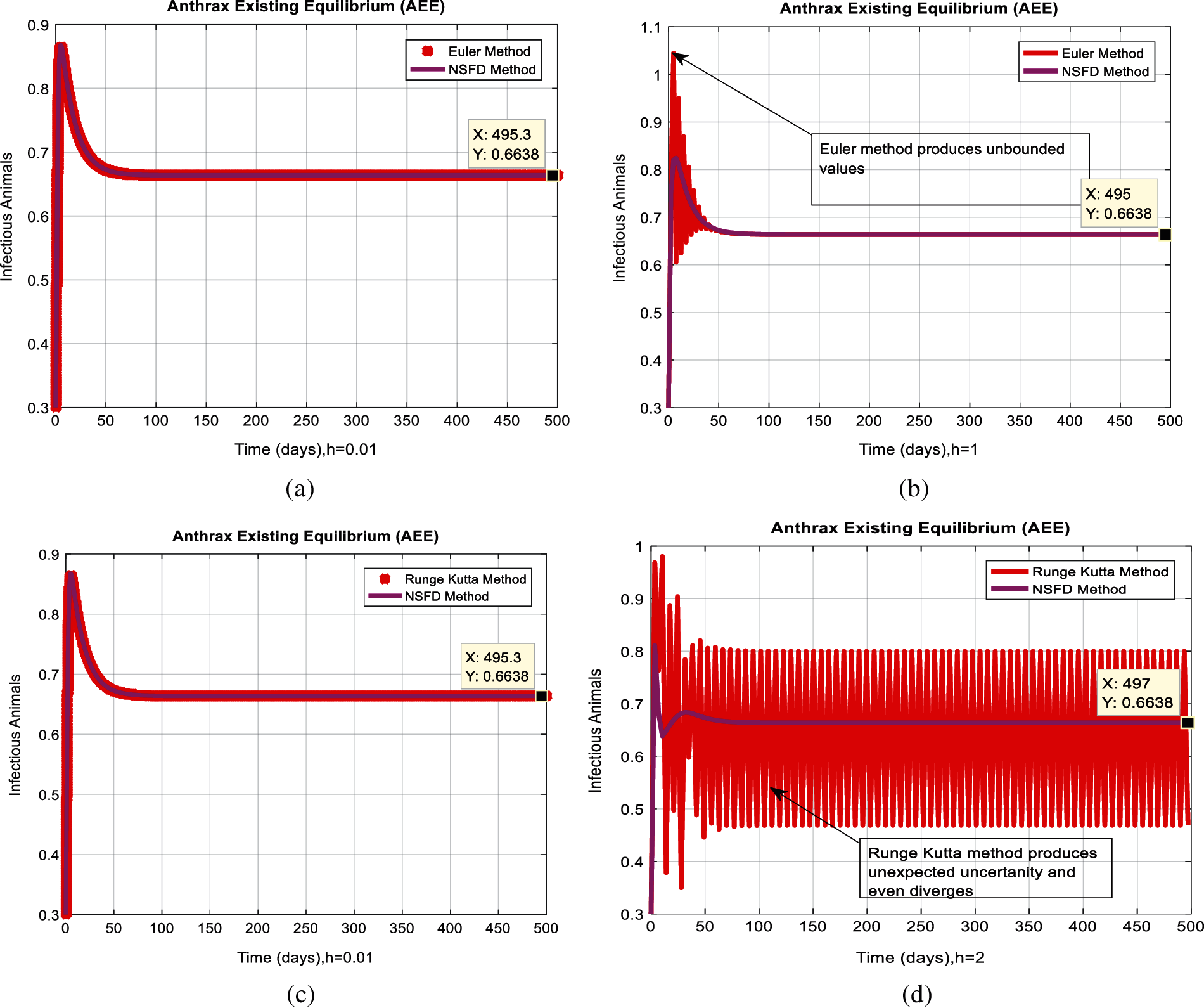
Figure 6: Combined behaviors of NSFD with Euler and Runge Kutta at different step sizes (a) Converges to true equilibria of NSFD and Euler methods for the infected population at anthrax existing equilibrium when h = 0.01 (b) Euler method diverges and produce negativity at h = 1 (c) Converges to true equilibria of NSFD and Runge Kutta methods for the infected population at anthrax existing equilibrium when h = 0.01 (d) Runge Kutta method diverges, produce negativity, and even fluctuation at h = 2
4 Results and Concluding Remarks
In Figs. 2a and 2b, we used the command-built software ODE-45 to simulate the behavior of the model at any time t. In Figs. 3a and 3b, the behavior of the computer method like Euler at different time step sizes are presented in which we can analyze the said method is converges for the small-time step size. In Figs. 4a and 4b, the second important method like Runge Kutta is also diverged and depends upon time step size. In meanwhile, Figs. 5a and 5b, is the true sense results simulates by non-standard finite difference method at any time step size. This computer method has the advantage over the other two methods like Euler and Runge Kutta. Figs. 6a and 6d is the ethnicity of the proposed computer method. Independent of time step size, low-cost and effective technique. Through the study, anthrax disease modeling is analyzed along with analytical approaches and computer techniques. The model is based on four compartments two humans (Susceptible and infected) and two related to dead bodies and spores’ germs (bacteria). The human compartment along with positivity, boundedness, equilibria, reproduction number, and local stability is studied rigorously. In the future, we could extend this type of modeling to other complex epidemiological models and their branches.
Acknowledgement: Thanks, our families and colleagues who supported us morally.
Funding Statement: The author(s) received no specific funding for this study.
Conflicts of Interest: The authors declare that they have no conflicts of interest to report regarding the present study.
1. C. Mackey and C. Kribs, “Can scavengers save zebras from anthrax? A modeling study,” Infectious Disease Modelling, vol. 6, no. 2, pp. 56–74, 2021. [Google Scholar]
2. E. B. Baloba, B. Seidu and C. S. Bornaa, “Mathematical analysis of the effects of controls on the transmission dynamics of anthrax in both animal and human populations,” Computational and Mathematical Methods in Medicine, vol. 20, no. 3, pp. 1–14, 2020. [Google Scholar]
3. E. Stella, L. Mari, J. Gabrieli, C. Barbante and E. Bertuzzo, “Permafrost dynamics and the risk of anthrax transmission: A modelling study,” Scientific Reports, vol. 10, no. 01, pp. 01–12, 2020. [Google Scholar]
4. S. Rezapour, S. Etemad and H. Mohammadi, “A mathematical analysis of a system of caputo-fabrizio fractional differential equations for the anthrax disease model in animals,” Advances in Difference Equations, vol. 481, no. 02, pp. 01–30, 2020. [Google Scholar]
5. A. M. Croicu, “An optimal control model to reduce and eradicate anthrax disease in herbivorous animals,” Bulletin of Mathematical Biology, vol. 81, no. 1, pp. 235–255, 2019. [Google Scholar]
6. J. P. Gomez, D. M. Nekorchuk, L. Mao, S. J. Ryan, J. M. Ponciano et al., “Decoupling environmental effects and host population dynamics for anthrax: A classic reservoir-driven disease,” Plos One, vol. 13, no. 12, pp. e0208621, 2018. [Google Scholar]
7. S. Mushayabasa, T. Marijani and M. Masocha, “Dynamical analysis and control strategies in modeling anthrax,” Computational and Applied Mathematics, vol. 36, no. 3, pp. 1333–1348, 2017. [Google Scholar]
8. C. M. S. Roy, P. V. D. Driessche and A. Yakubu, “A mathematical model of anthrax transmission in animal populations,” Bulletin of Mathematical Biology, vol. 79, no. 2, pp. 303–324, 2017. [Google Scholar]
9. S. Mushayabasa, “Dynamics of an anthrax model with distributed delay,” Acta Applicandae Mathematicae, vol. 144, no. 1, pp. 77–86, 2016. [Google Scholar]
10. W. Chen, G. Alain and R. Angel, “Modeling the logistics response to a bioterrorist anthrax attack,” European Journal of Operational Research, vol. 254, no. 2, pp. 458–471, 2016. [Google Scholar]
11. B. Pantha, J. Day and S. Lenhart, “Optimal control applied in an Anthrax epizootic model,” Journal of Biological Systems, vol. 24, no. 04, pp. 495–517, 2017. [Google Scholar]
12. B. Gutting, “Deterministic models of inhalational anthrax in New Zealand white rabbits,” Biosecurity and Bioterrorism: Biodefense Strategy, Practice and Science, vol. 12, no. 01, pp. 29–41, 2014. [Google Scholar]
13. D. J. A. Toth, A. V. Gundlapalli, W. A. Schell, K. Bulmahn, T. E. Walton et al., “Quantitative models of the dose-response and time course of inhalational anthrax in humans,” PLoS Pathogens, vol. 9, no. 8, pp. e1003555, 2013. [Google Scholar]
14. J. Day, A. Friedman and L. S. Schlesinger, “Modeling the host response to inhalation anthrax,” Journal of Theoretical Biology, vol. 276, no. 1, pp. 199–208, 2011. [Google Scholar]
15. D. A. Wilkening, “Modeling the incubation period of inhalational anthrax,” Medical Decision Making: An International Journal of the Society for Medical Decision Making, vol. 28, no. 4, pp. 593–605, 2008. [Google Scholar]
16. H. Li, S. D. Soroka, T. H. TaylorJr., K. L. Stamey, K. W. Stinson et al., “Standardized mathematical model based and validated in vitro analysis of anthrax lethal toxin neutralization,” Journal of Immunological Methods, vol. 333, no. 1-2, pp. 89–106, 2008. [Google Scholar]
17. P. R. Pittman, P. H. Gibbs, T. L. Cannon and A. M. Friedlander, “Anthrax vaccine: Short-term safety experience in humans,” Vaccine, vol. 20, no. 5-6, pp. 972–978, 2001. [Google Scholar]
18. P. R. Furniss and B. D. Hahn, “A mathematical model of an anthrax epizoötic in the Kruger National Park,” Applied Mathematical Modelling, vol. 5, no. 3, pp. 130–136, 1981. [Google Scholar]
19. P. V. D. Driessche, “Reproduction numbers of infectious disease models,” Infectious Disease Modelling, vol. 2, no. 3, pp. 288–303, 2017. [Google Scholar]
20. M. Helikumi, P. O. Lolika and S. Mushayabasa, “Implications of seasonal variations, host and vector migration on spatial spread of sleeping sickness insights from a mathematical model,” Informatics in Medicine Unlocked, vol. 24, no. 01, pp. 01–12, 2021. [Google Scholar]
21. G. F. Webb, “A silent bomb: The risk of anthrax as a weapon of mass destruction,” Proceedings of the National Academy of Sciences of the United States of America, vol. 100, no. 8, pp. 4355–4356, 2003. [Google Scholar]
22. P. Afshar, M. T. Hedayati, N. Aslani, S. Khodavaisy, F. Babamahmoodi et al., “First autochthonous coinfected anthrax in an immunocompetent patient,” Case Reports in Medicine, vol. 2015, no. 5, pp. 1–5, 2015. [Google Scholar]
23. S. A. Hashemi, A. Azimian, S. Nojumi, T. Garivani, S. Safamanesh et al., “A case of fatal gastrointestinal anthrax in north eastern Iran,” Case Reports in Infectious Diseases, vol. 2015, no. 2, pp. 1–2, 2015. [Google Scholar]
24. S. Osman and O. D. Makinde, “A mathematical model for coinfection of listeriosis and anthrax diseases,” International Journal of Mathematics and Mathematical Sciences, vol. 2018, no. 3, pp. 1–14, 2018. [Google Scholar]
25. R. Brookmeyer, E. Johnson and S. Barry, “Modelling the incubation period of anthrax,” Statistics in Medicine, vol. 24, no. 04, pp. 531–542, 2005. [Google Scholar]
26. V. A. Karginov, T. M. Robinson, J. Riemenschneider, B. Golding, M. Kennedy et al., “Treatment of anthrax infection with combination of ciprofloxacin and antibodies to protective antigen of bacillus anthracis,” FEMS Immunology & Medical Microbiology, vol. 40, no. 1, pp. 71–74, 2004. [Google Scholar]
27. C. L. Loving, M. Kennett, G. M. Lee, V. K. Grippe and T. J. Merkel, “Murine aerosol challenge model of anthrax,” Infection and Immunity, vol. 75, no. 6, pp. 2689–2698, 2007. [Google Scholar]
28. V. Radosavljevic, D. Radunovic and G. Belojevic, “Epidemics of panic during a bioterrorist attack– A mathematical model,” Medical Hypotheses, vol. 73, no. 3, pp. 342–346, 2009. [Google Scholar]
29. A. Raza, A. Ahmadian, M. Rafiq, S. Salahshour and M. Ferrara, “An analysis of a nonlinear susceptible-exposed-infected-quarantine-recovered pandemic model of a novel coronavirus with delay effect,” Results in Physics, vol. 21, no. 01, pp. 01–07, 2021. [Google Scholar]
30. A. Raza, A. Ahmadian, M. Rafiq, S. Salashour, M. Naveed et al., “Modeling the effect of delay strategy on transmission dynamics of HIV/AIDS disease,” Advances in Difference Equations, vol. 663, no. 01, pp. 01–19, 2020. [Google Scholar]
31. N. Ahmed, A. Raza, M. Rafiq, A. Ahmadian, N. Batool et al., “Numerical and bifurcation analysis of SIQR model,” Chaos Solitons and Fractals, vol. 150, no. 01, pp. 01–15, 2021. [Google Scholar]
32. J. E. M. Diaz, A. Raza, N. Ahmed and M. Rafiq, “Analysis of a nonstandard computer method to simulate a nonlinear stochastic epidemiological model of coronavirus-like diseases,” Computer Methods and Programs in Biomedicine, vol. 204, no. 01, pp. 01–10, 2021. [Google Scholar]
33. A. Akgul, M. S. Iqbal, U. Fatima, N. Ahmed, Z. Iqbal et al., “Optimal existence of fractional order computer virus epidemic model and numerical simulations,” Mathematical Methods in the Applied Sciences, vol. 7437, no. 01, pp. 01–13, 2021. [Google Scholar]
34. U. Fatima, D. Baleanu, N. Ahmed, S. Azam, A. Raza et al., “Numerical study of computer virus reaction diffusion epidemic model,” Computers, Materials & Continua, vol. 66, no. 3, pp. 3183–3194, 2021. [Google Scholar]
35. A. Raza, A. Ahmadian, M. Rafiq, S. Salahshour and I. R. Laganà, “An analysis of a nonlinear susceptible-exposed-infected-quarantine-recovered pandemic model of a novel coronavirus with delay effect,” Results in Physics, vol. 21, no. 01, pp. 01–07, 2021. [Google Scholar]
36. W. Shatanawi, A. Raza, M. S. Arif, M. Rafiq, M. Bibi et al., “Essential features preserving dynamics of stochastic dengue model,” Computer Modeling in Engineering & Sciences, vol. 126, no. 1, pp. 201–215, 2021. [Google Scholar]
37. A. Raza, M. S. Arif, M. Rafiq, M. Bibi, M. Naveed et al., “Numerical treatment for stochastic computer virus model,” Computer Modeling in Engineering & Sciences, vol. 120, no. 2, pp. 445–465, 2019. [Google Scholar]
38. M. S. Arif, A. Raza, K. Abodayeh, M. Rafiq and A. Nazeer, “A numerical efficient technique for the solution of susceptible infected recovered epidemic model,” Computer Modeling in Engineering & Sciences, vol. 124, no. 02, pp. 477–491, 2020. [Google Scholar]
39. W. Shatanawi, A. Raza, M. S. Arif, M. Rafiq, M. Bibi et al., “Essential features preserving dynamics of stochastic dengue model,” Computer Modeling in Engineering & Sciences, vol. 126, no. 1, pp. 201–215, 2021. [Google Scholar]
40. M. A. Noor, A. Raza, M. S. Arif, M. Rafiq, K. S. Nisar et al., “Non-standard computational analysis of the stochastic COVID-19 pandemic model: An application of computational biology,” Alexandria Engineering Journal, vol. 61, no. 1, pp. 619–630, 2022. [Google Scholar]
41. K. Abodayeh, A. Raza, M. S. Arif, M. Rafiq, M. Bibi et al., “Numerical analysis of stochastic vector borne plant disease model,” Computers, Materials & Continua, vol. 62, no. 3, pp. 65–83, 2020. [Google Scholar]
42. K. Abodayeh, A. Raza, M. S. Arif, M. Rafiq, M. Bibi et al., “Stochastic numerical analysis for impact of heavy alcohol consumption on transmission dynamics of gonorrhoea epidemic,” Computers, Materials & Continua, vol. 62, no. 3, pp. 1125–1142, 2020. [Google Scholar]
 | This work is licensed under a Creative Commons Attribution 4.0 International License, which permits unrestricted use, distribution, and reproduction in any medium, provided the original work is properly cited. |