DOI:10.32604/iasc.2022.022654
| Intelligent Automation & Soft Computing DOI:10.32604/iasc.2022.022654 | |
| Article |
Automatic Human Detection Using Reinforced Faster-RCNN for Electricity Conservation System
Faculty of Engineering and Technology, SRM Institute of Science and Technology, Kattankulathur, Chennai, 603203, India
*Corresponding Author: S. Ushasukhanya. Email: ushasukhanya@gmail.com
Received: 14 August 2021; Accepted: 15 September 2021
Abstract: Electricity conservation systems are designed to conserve electricity to manage the bridge between the high raising demand and the production. Such systems have been so far using sensors to detect the necessity which adds an additional cost to the setup. Closed-circuit Television (CCTV) has been installed in almost everywhere around us especially in commercial places. Interpretation of these CCTV images is being carried out for various reasons to elicit the information from it. Hence a framework for electricity conservation that enables the electricity supply only when required, using existing resources would be a cost effective conservation system. Such a framework using a deep learning model based on Faster-RCNN is developed, which makes use of these CCTV images to detect the presence or absence of a human in a place. An Arduino micro-controller is embedded to this framework which automatically turns on/off the electricity based on human's presence/absence respectively. The proposed approach is demonstrated on CHOKE POINT dataset and two real time datasets which images from CCTV footages. F-measure, Accuracy scores (AUC score) and training time are the metrics for which the model is evaluated. An average accuracy rate of 82% is obtained by hyper-parameter tuning and using Adam optimization technique. This lays the underpinning for designing automatic frameworks for electricity conservation systems using existing resources.
Keywords: Deep neural network; Faster-RCNN; Resnet-50; Hyperparameter tuning; Arduino
Electricity conservation is one of the most demanding tasks in many countries of the globe. Many of the existing products are being replaced by products which consume less electrical energy. Though various researches are being carried out in inventing new ways to conserve electricity, the challenge still persists [1]. Among the several methods carried out to bridge the gap between the availability and demand of the resource, one of the efficient ways to conserve electricity would be to use the resource only when it is actually needed. This study uses an automated system that enables and disables electricity only when a human being is being detected/undetected in a frame respectively. The system uses the input from live surveillance camera footages to detect the human beings in the frame. As the need for safety and security of the people and infrastructure is increasing every day, closed circuit television (CCTV) cameras are being installed everywhere. Thus, without any additional devices like sensors, the proposed system makes use of prevailing CCTV cameras and the live footages of it, to track human beings and their location, thereby automatically enabling the electrical power only in the location where human is detected. Electricity is turned off in the locations where human is unavailable or undetected.
Object detection is an active field of research over the recent years [2]. Automating the process of detecting objects in live surveillance footage certainly depends on the magnitude of the algorithms being used. Computer vision and Machine learning (ML) techniques have achieved remarkably great heights in object detection. Due to its inability to extract complex features of the objects and the inability to handle large data, ML techniques have failed in certain fields [3]. However, Deep learning (DL) techniques can handle enormous data to extract high level features which are mandatory for processing real time surveillance footages. Deep learning has proved its efficiency in detection, classification [4], recognition [5] of objects in images. Target localization [6] is another important aspect where ML has excelled.
This study develops a deep learning model based on Faster-RCNN is developed, which makes use of these CCTV images to detect the presence or absence of a human in a place. An Arduino micro-controller is embedded to this framework which automatically turns on/off the electricity based on human's presence/absence respectively. The proposed approach is demonstrated on CHOKE POINT dataset and two real time datasets which images from CCTV footages. F-measure, Accuracy scores (AUC score) and training time are the metrics for which the model is evaluated. An average accuracy rate of 82% is obtained by hyper-parameter tuning and using Adam optimization technique.
An automated human detection system is developed using Deep Regional based classifier, Faster R-CNN to detect human beings and their location in surveillance videos. Hence related survey is discussed in the following sub sections.
2.1 Conventional Computer Vision Techniques
With the increasing security threats, CCTV s are being installed everywhere for surveillance purpose. Enormous videos and frames are generated from these CCTV footages are being used in various applications of object detection. Like human beings, computer vision plays a major role in understanding and detecting objects in videos or frames [7]. The steps involved in detecting the objects using conventional methods are pre-processing, segmentation, feature extraction, object recognition and structural analysis [8]. Machine learning model integrates most of these steps, thereby saves time with increased accuracy in prediction. Object detection in frames of indoor to outdoor environment, underground to satellite images is been extensively carried out with CNN and its variants. A major limitation of machine learning technique is the capacity of data that it can handle. As this system requires enormous training of the model and learning of complex features for better prediction, machine learning models fails to perform well. Thus Deep learning comes into comes into the picture of our system.
2.2 Deep Learning Based Computer Vision Techniques
Deep learning techniques (especially CNN) have been used extensively in image analysis over the past few decades [9]. CNN is restricted to only detect the objects, but not its location. As our system demands the location of the human being, regional based classifier is used. Most of the conventional methods are based on the model developed by Szegedy et al. [10]. The model uses five different training procedures to figure out the object locations in the frames. Similarly another DNN model was developed by Brody et al. which produces bounding boxes around the objects in the frames [11]. Though efficiency degradation due to poor fine-grained categorization is overcome by pose-normalization, these methods still require bounding-box hypotheses and hence zhang et al. proposed a bottom-up strategy in Deep CNN.
Another model that has gained attraction in recent years is fast R-CNN which has yielded promising results in object detection. As RCNN is computationally expensive and extremely slow, a variant of it called fast RCNN was developed. Fast-RCNN discards the usage of SVMs in classification and bounding box regression, by replacing it with a Softmax classifier. Hence, the former two models are combined into one single model, which is to be trained once. Secondly, Fast RCNN makes use of a bounding box regressor to optimize the region proposals, which yields high accuracy and also speeds up the training process [12]. Although Fast R-CNN is an improved version of RCNN, the proposal approach/network and the detection network are separated in both R-CNN and Fast R-CNN. This is the main drawback, especially when SS algorithm has a false negative; it directly affects the detection network [13].
To end this, Faster RCNN was developed which trains both region proposals and classification modules with end to end joint training. Wang et al. [14] designed a system using Faster R-CNN for detecting dairy goats in surveillance videos. Silhouettes extraction and aggregation of the differences between subsequent frames of an action sequence is done to extricate the key frames. Foreground segmentation is also incorporated to detect the incomplete dairy goats. This is done by fusing the local colour intensity with spatio-temporal neighbourhood similarity function by the background model. Finally, the region proposals are also combined with the detection results. The achieved 92.57% of accuracy shows that the method is highly preferable than the conventional Faster R-CNN but the detecting speed still falls behind for a real-time video processing.
Though faster R-CNN improves the prediction accuracy, the model has to be optimized for reducing the training time, to avoid over-fitting which subsequently enhances the overall efficiency. A similar system was developed by Zhou et al. [15] for marine organism detection and recognition. Data augmentation is done by perspective transformation and a four-step alternate training method with SGD is used for the training process of RPN. The achieved experimental results confirm the enhanced robustness of Faster R-CNN to various aspects of the marine environment.
Also, a model to detect maize seedlings was designed by Quan et al. [16] by building a field robot platform. 62.485 images under various conditions like full cycle, multi-weather and full angle were obtained to classify the seedlings into appropriate classes on a GPU platform. Feature extraction is done by using the similarity variable or image matching method. Classification is done by Faster R-CNN with optimized VGG-19 achieving the best precision between 90% to 95%. Humbrid et al. [17] proposed a neural network model with a novel mapping from decision trees to deep neural networks. The mapping produces a network with a specific number of hidden layers, neurons per hidden layer, and a set of initial weights to optimize the architecture at lower cost. The Adam optimizer [18] is used to minimize the cost function, which is mean squared error (MSE) for regression, and cross entropy with for classification. The author has stated that DJINN could be used for image analysis tasks after convolutional layers extract the important features.
2.3 Home Automation for Electricity Conservation
Home automation and energy measurements have always been an interesting topic of research. Various microcontrollers are used for these applications depending upon the requirements. Among the various existing systems, a system was developed by Srividyadevi to estimate the energy of the load given in a laboratory using a data acquisition board (DAQ) connected to a personal computer. Arduino digitally measures the power consumed and displays it graphically using Meguno link software. Another energy management system was developed by Qinran Hu with sensitive technology and Classification algorithms. All of these systems are found to make use of the sensors to detect human beings in the spot. This actually increases the cost of the system especially when it used in large real-time applications. Hence our work has designed an optimized system that makes use of the prevailing resources (CCTV cameras) for detecting human beings and to subsequently manage the electric power resource.
Following are the few major issues that have been inferred from the survey to address it in our work.
• Hyperparameter tuning is major concern in Deep Learning, which results in high training time. This is considerably reduced using Enhanced orthogonal array tuning method (E-OATM) without impacting the accuracy of the network.
• Overfitting impacts heavily on the accuracy of the Deep Neural Network as it is a complex model which is avoided by regularization and dropout techniques.
• Eventually, there has not been any framework designed so far using the existing resources (without sensors) for electricity conservation and to design the same is our target eventually.
The framework takes the input from existing CCTV images of CHOKEPOINT dataset. It consists of 64,204 frames in three distinct indoor environments. All the images are with a resolution of 800 × 600 pixels. 70% of images in each class contain positive images (Images with human) whereas the remaining 30% has negative images (images without human). The system is evaluated with a real time CCTV footage where the frame rate per second is 6. 80% of the frames in CHOKEPOINT dataset are considered for training set and the remaining 20% for test set. Fig. 1 shows the positive and negative frames.

Figure 1: Positive and negative frames in all three environments of CHOKEPOINT dataset
Manual whisker annotator is an open source tool used to annotate the images of the dataset with human. The labelled images are exported to an extensible Markup Language (XML) file. Out of 64,204 CHOKEPOINT images with and without human, around 47,204 ROI s are generated with human. Finally we produce a total of 37.764 images of the positive class for training and the remaining 9440 positive class images for testing. Further, the images are zero-centred to increase the learning speed which is followed by the normalization process. The inputs are then resized to 256 × 256 × 3 for better feature description.
Image classification is done by Faster R-CNN which is an advanced version of RCNN and Fast-RCNN. The network combines a unique Region Proposal Network (RPN) which proposes regions with Fast RCNN that makes use of the RPN proposed regions to detect an object. The algorithm for the entire framework is given in Fig. 2.

Figure 2: Pseudocode of conventional and reinforced algorithms. (a) Conventional algorithm, (b) Reinformed algorithm
In this network, CNN is used for RPN rather than using selective search (SS) in earlier models. RPN's responsibility is to output a set of rectangular object proposals for an input image of any size. The model attentively helps the classifier in finding out the regions that it should consider. The input image is run through 2 modules: First is the RPN which generates object regions and second is the classification of the region proposals which is done by fast R-CNN. The entire process is modelled with a fully convolutional network.
The Detection network is fed with inputs from both feature network and the RPN to generate the final class and bounding box. The network consists of two common stacked layers shared by a classification layer and a bounding box regression layer along with four FC layers. The features of the images are cropped based on the bounding boxes to aid classification.
4.3.3 Convolutional Neural Networks
Various transfer learning and customized neural networks like AlexNet, VGGNet, ResNet, GoogleNet, DenseNet etc have been implemented so far in classification of surveillance frames. The training time in Alexnet took around 40 days for the model to learn with the error rate being less than 17.2%. VGG 19 was then implemented to reduce the trainable parameters of Alexnet which in turn increases the learning speed of the architecture. It took around 33 days for the network to learn with an error rate of 16.3%. Both these networks face Vanishing gradient problem where the gradients decrease and finally reaches zero as we move in the reverse direction of the network. This is called as decay of information through back propagation which is avoided in ResNet by implementing residual connections with the initial layers. There are many variations of ResNet like ResNet-18, ResNet-34, ResNet-50, ResNet-101, ResNet-152 etc out of which ResNet-50 is more suited on real time applications by all means.
All these networks are optimized to increase the overall efficiency of the network. Among the various efficiency determining parameters, one important factor is the training time reduction and to reduce the training time, optimal set of parameters should be determined at the earliest. All these are possible by tuning the hyper-parameter of the network. The biggest challenge of DNN is the hyper-parameter tuning because of its large number and its dependency on the configuration. For instance, the grid search is a time consuming process while the random search is poor in reaching out to the global minimum when compared to grid search [19]. Though there are many automated tuning methods, all these fail in either of the above specified two drawbacks.
To overcome these issues especially to reduce the training time without disturbing the prediction accuracy of the network, Xiang Zhang suggested an orthogonal array tuning method to tune the hyper-parameters of CNN. Inspired by this, we have taken the same approach with little modification of the existing one for our automated system. The approach considers more number of hyper-parameters for tuning as the considered hyper-parameters by Xiang Zhang is insufficient for real-time scenarios.
4.3.4 Proposed Network Structure
As transfer learning is not best suited for real time applications, a modified architecture of Resnet-50 is used for this system. The reason behind choosing Resnet-50 is to avoid vanishing gradient problem. Also the convolutional layers of ResNet are tuned with the optimal values which are found using E-OATM method. The detailed process of the entire system is described in Fig. 3.

Figure 3: Working model of the proposed framework
The convolutional layers with relu activation function and max pooling in the initial stage receives the input image and outputs the feature maps. Min-max normalization is then done to eradicate the lighting effect in the images. It is done pixel by pixel based on the following formula
RPN is the series of convolution layers which has a structure of Resnet 50. To avoid exploding or vanishing gradient issues, the weights of the layers have been initialized by
where “a” is the weight matrix, “I” is the input, “Y” is the output and “n” is the total number of elements. The weights are initialized using He initialization scheme with uniform distribution as this initialization works well for relu activations. The initialization scheme is based on
where V is the variance, W is the weights and fanin represents the units in the previous layers. As the activation function is scaled in the back propagation also, the mean of the fans is not calculated. The initial weights of the layers lie in the range of 0.01 to 0.062. The kernel size of the initial convolution and pooling layers are set to 7 × 7 and 3 × 3 respectively with stride 2.
This is followed by the first, second and third residual blocks with three convolutional layers in each block till 45 layers in 4 states with an identity connection in between the layers. A batch normalization layer is added after each activation layer to accelerate the learning process. To address the first objective of our work, the high training time is considerably reduced by finding a set of optimal parameters and hyperparameters to tune the network which is done based on E-OATM. OATM is a method whose entries are from a pre-determined set of values organized in a specific format. It is actually a representative subset of the exhausting full set of elements. Factors represents the parameters and hyper-parameters and the levels define its corresponding values. We have considered six hyper-parameters and two model parameters for tuning to minimize the loss function with respect to multiple variables at less cost.
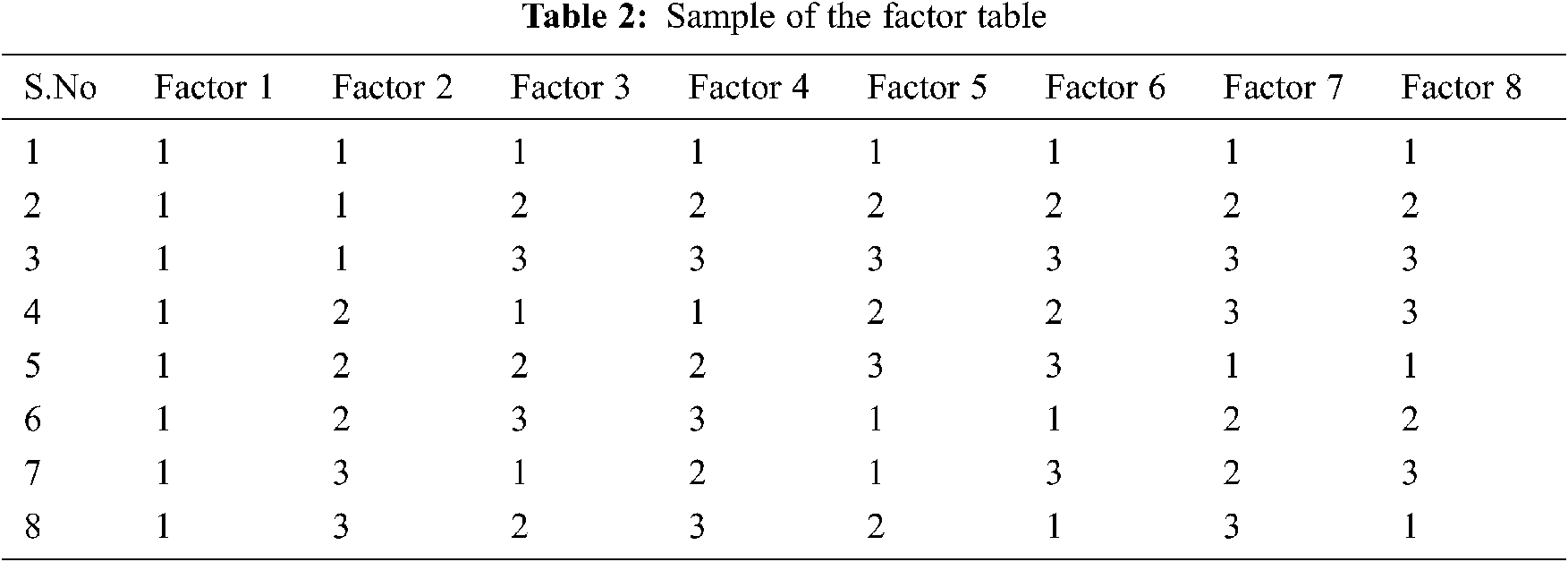
CNN is trained with the hyper-parameters values generated according to the factor table of Taguchi method. 64, 64 and 256 are the kernel sizes with 1 × 1, 3 × 3 and 1 × 1 convolutions in the first residual block of Resnet 50. The factors are initialized with the following values listed in Tab. 1 for training purpose.

The orthogonal array table is generated using Weibull ++ with K factors, H levels and M rows have 18 observations. The factor table has 18 rows and hence a sample of the factor table for the selected six factors is given in Tab. 2.
The identity connection sums the input with the output of each and every residual block to approximate the final function such that the output is close to the input function. It is followed by the function
where A is the output function of residual block i, F(x) is the output of the third layer of the residual block 1 and x is the input given. Finally, the network uses an average pooling layer and a dense layer of 1000 neurons which is parameterized by the weight matrix W50 and a bias vector b50.
A small sliding window now slides over the feature map of the dense layer of ResNet to generate K region proposals. The network yields foreground anchors of the objects with 1:1, 1:2, and 2:1 aspect ratio. All the samples with IoU (Intersection over union) > 0.7 and with IoU < 0.7 are considered to be positive and negative samples, respectively. Non-Maximum suppression (NMS) is then applied to reduce the overlapping regions generated by RPN. The resulting 2000 proposals are ranked based on the object scores and the top ranked proposals are used for training initially followed by the low ranked proposals. Lastly, the unique layers of Fast R-CNN are also fine-tuned with the learning rate of 0.001 to process the input ROIs of the RPN. The fixed-length feature vector of each ROI is fed into the dense layers, where the last prediction layers of Resnet-50 are replaced with our prediction layers PL_1 and PL_2 which is followed by the softmax layer and the regression layer.
4.3.5 Training and Testing Process
The model is now created and it has to be learned using the training dataset. Hyperparameter tuning is to be done to control the learning process for which the optimal values are to be determined from the set of values considered. Hence the model is trained with the all the values based on the factor table generated by the Taguchi method. After training, the model is tested with few images of the test data set. These are passed into the model and the prediction accuracy, F-Score of the model is evaluated for each set of values generated by the factor table. The range analysis for all the seven factors is calculated and the highest accuracy row with its values is considered to be the optimal value to tune the model. As it difficult to explicitly display the accuracy metrics of all 18 levels, a few levels are shown in Tab. 3.

The highest accuracy is obtained in the sixth level and hence the values of the parameters and the hyper-parameters in the sixth level are considered to be the optimal one to tune the model. The model is iterated on these optimal values with learning rate 0.01, Momentum 0.99, Filter size 3 × 3 which is reduced to 1 × 1 at each level and the number of neurons used in each hidden layer is 128. To address the second objective of our work, L2 regularization technique is used with a weight decay of 0.01 and dropout of 0.20 is used to avoid over fitting of the model. As the dataset contains sufficient number of images, data scarcity is not an issue for our work. The model is then iterated for 398 epochs with a batch size of 128 images and an average accuracy of six iterations is considered to be the final value. All these optimal values are obtained in 18 iterations whereas it would take 28,211 combinations in a grid search.
The training time of this takes around 1722 s whereas it takes 28,269 s in grid search approach. Therefore, it saves around 85% of the training time thereby yielding an accuracy of 88.3%. RPN is trained using a multi-task loss function calculated using
where x and Px constitutes the anchor numbers and its predicted probability respectively, the ground truth label which is indicated by Px* is equal to one for a human present sample and 0 otherwise. Qx and Qx* indicates the coordinates of predicted bounding box and ground-truth bounding box for a positive anchor respectively. The two normalization factors Ncls and Nreg are set to 256 and 2400 which are balanced by λ value of 10. The unique layers of Fast R-CNN are also fine-tuned with the learning rate of 0.001 and the coordinates of the anchor are given by the following equations [20]:
where the width, height centre coordinates and the corresponding values of the bounding boxes are represented by w, h, x, y, x0 and x* respectively. The same annotation method is used for y, w, and h. Finally, the regions with a classification confidence score greater than 0.7 is considered as human and non-human otherwise. The NMS threshold is set to 0.3 and the classification of images with bounding boxes is done specifying the location of the human. The classification loss Lcls over two objects is estimated by the log loss function and the regression loss Lreg using the robust regression loss function.
The model is then optimized with Adam optimization technique with a learning rate set to 0.001 which increases the accuracy from 88.3% to 89.9%.
The model is validated on a real-time dataset (Dataset 2) where a surveillance video of a faculty room in an educational institution is considered, as shown in Fig. 4. The duration of the video is 150 min which is converted to 6 frames per second. On total, it yields about 54000 images. The model yields about 86% of accuracy in classifying the frames with and without human.
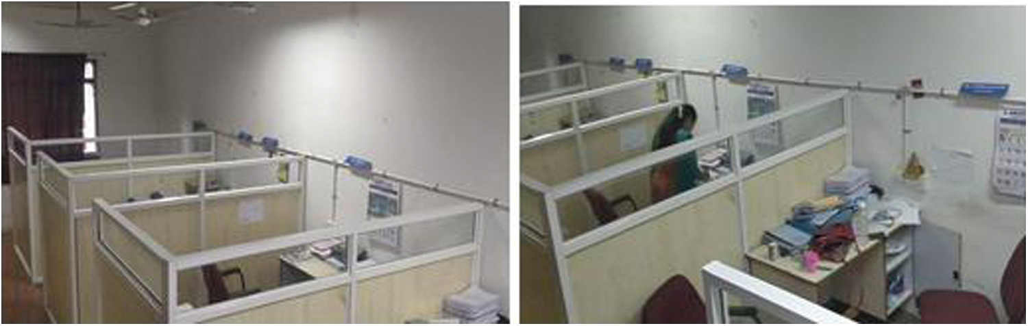
Figure 4: Positive and negative frames in real time CCTV video
The reduction in percentage when compared to the CHOKEPOINT dataset is due to the poor lighting conditions of the surveillance video.
4.5 Establishing Control Over Electric Power Supply
The system uses an arduino micro-controller for managing the electric power supply in an indoor environment. Arduino has been used in many applications as it is based on simplifies version of C/C++ which is simpler and quite inexpensive. As Arduino MEGA 2560 has more digital and analog pins that can enable the control of more loads, it has been used in this system. The output of the classifier is connected to this system whereby the controller is programmed to enable the power supply whenever a human is detected and to disable it otherwise. This is done sequentially to all the frames of the datasets with a time delay of 4.3 s.
The CHOKEPOINT dataset has been divided into three classes where the first class has 21,402 images, second class contains 21,402 images and the third class contains 21,400 images. Each class has a training set comprising of 80% of the frames and the testing set with 20% of frames. The model is trained with original Resnet-50 and the results are shown in Tab. 4.

The results of optimized Resnet-50 on 3 classes of the CHOKEPOINT dataset is shown in Tab. 5.

The receiver operating characteristic curve (ROC) curve is plotted against both the models on the CHOKEPOINT dataset and its accuracy is shown in Fig. 5.
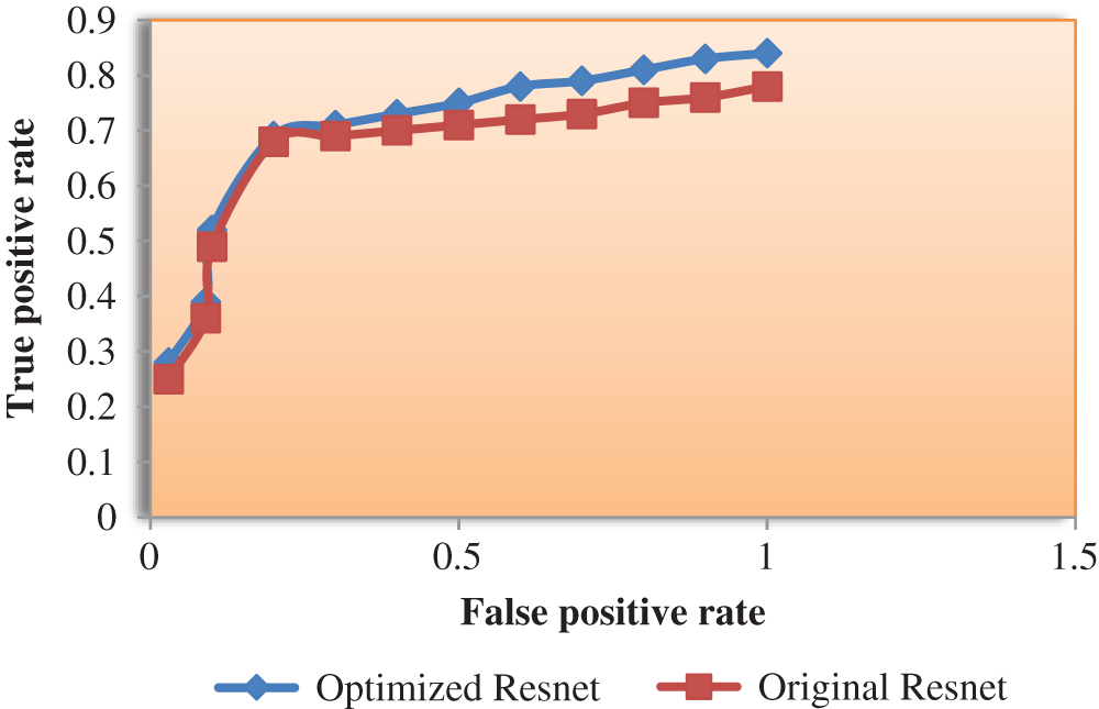
Figure 5: ROC curve for the Original Resnet-50 vs. Optimized Resnet-50 on CHOKEPOINT dataset
Both the original and the modified models are validated on real-time dataset and the results are shown in Tabs. 6 and 7.


The ROC curve for the surveillance dataset is plotted for both the models and the accuracy is given in Fig. 6.
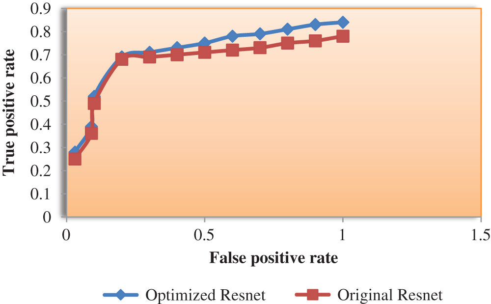
Figure 6: ROC curve for the Original Resnet-50 vs. Optimized Resnet-50 on Real-time dataset
The results of faster-RCNN which identifies human with the location in an indoor environment in all the datasets are shown in Fig. 7.
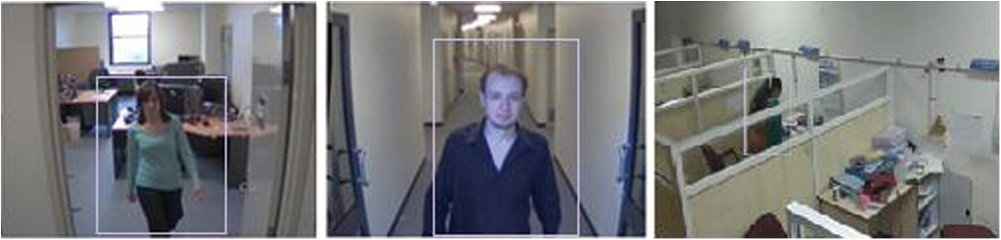
Figure 7: Identification of human with location in both the datasets
Thus the location of the human's presence is identified by the classifier which is then connected to the microcontroller to enable the power supply. The controller disables the power supply when human is unavailable in the room and the results are shown in Fig. 8 thereby addressing the last objective of our work.
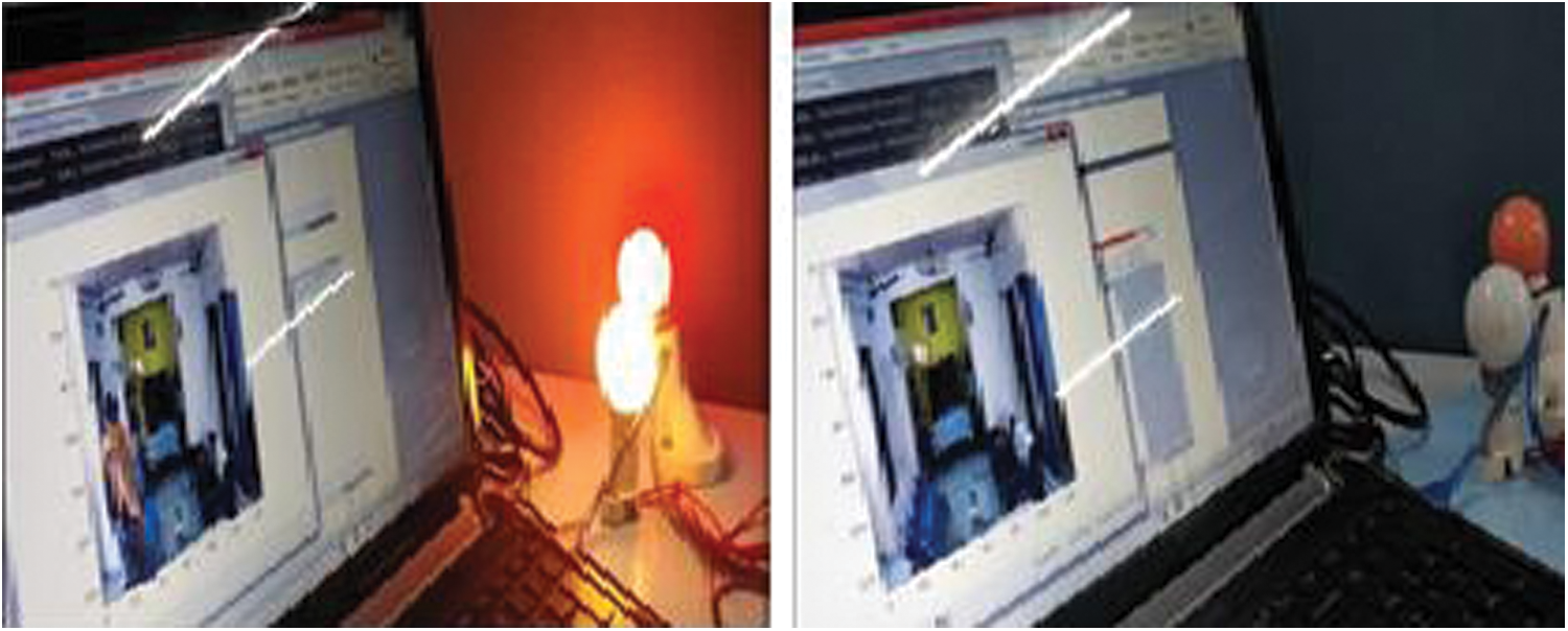
Figure 8: Electricity turned on and off when human is available and unavailable respectively
The electricity consumed on an average by a tubelight and a fan for 10 h is 1820 watts for the residential area shown above in Fig. 8, which in considerably reduced to 1560 watts using the proposed framework. This saves around 46.8 KWH on an average for a month which is nearly one quarter of the total electricity consumed for a month.
In conclusion, a framework for automatic electricity conservation system has been designed and developed for an indoor environment which is based on human's presence/absence. The framework is based on a deep learning model of faster R-CNN using Resnet-50. The major issues of a deep learning model like high training time, Overfitting and optimization is handled by E-OATM method, regularization, dropout, and Adam techniques respectively. However, the proposed system is well suited for an indoor environment and the outdoor environment is not taken into consideration. Weight pruning is another method which can be used in future to simplify the complex model created which is under implementation phase for the same electricity conservation system.
Funding Statement: The authors received no specific funding for this study.
Conflicts of Interest: The authors declare that they have no conflicts of interest to report regarding the present study.
1. A. Adelakun, A. A. Adewale, A. Abdulkareem and J. O. Olowoleni, “Automatic control and monitoring of electrical energy consumption using PIR sensor module,” International Journal of Scientific & Engineering Research, vol. 5, no. 5, pp. 493–496, 2014. [Google Scholar]
2. X. Jiang, A. Hadid, Y. Pang, E. Granger and X. Feng, (Eds“Deep Learning in Object Detection and Recognition,” Springer, Denmark, 2019. [Google Scholar]
3. N. Sharma, V. Jain and A. Mishra, “An analysis of convolutional neural networks for image classification,” Procedia Computer Science, vol. 132, pp. 377–384, 2018. [Google Scholar]
4. Z. Zhong, J. Li, Z. Luo and M. Chapman, “Spectral—Spatial residual network for hyperspectral image classification: A3-ddeep learning framework,” IEEE Transactions on Geoscience and Remote Sensing, vol. 56, no. 2, pp. 847–858, 2018. [Google Scholar]
5. J. Gao, T. Zhang, X. Yang and C. Xu, “P2t: Part-to-target tracking via deep regression learning,” IEEE Transactions on Image Processing, vol. 27, no. 6, pp. 3074–3086, 2018. [Google Scholar]
6. S. Wu, X. Zhao, H. Zhou and J. Lu, “Multi object tracking based on detection with deep learning and hierarchical clustering,” in 2019 IEEE 4th Int. Conf. on Image, Vision and Computing (ICIVCpp. 367–370, Xiamen, China, 2019. [Google Scholar]
7. D. H. Ballard and C. M. Brown, “Computer vision,” Prentice Hall, vol. 27, pp. 265–308, 1982. [Google Scholar]
8. H. Zakeri, F. M. Nejad and A. Fahimifar, “Image based techniques for crack detection, classification and quantification in asphalt pavement: A review,” Archives of Computational Methods in Engineering, vol. 24, no. 4, pp. 935–977, 2017. [Google Scholar]
9. A. Krizhevsky, I. Sutskever and G. E. Hinton, “Imagenet classification with deep convolutional neural networks,” Communications of the ACM, vol. 60, no. 6, pp. 84–90, 2017. [Google Scholar]
10. C. Szegedy, A. Toshev and D. Erhan, “Deep neural networks for object detection,” Advances in Neural Information Processing Systems, vol. 26, pp. 2553–2561, 2013. [Google Scholar]
11. B. Huval, A. Coates and A. Ng, “Deep learning for class-generic object detection,” NIPS’12: Proc. of the 25th Int. Conf. on Neural Information Processing Systems, vol. 25, pp. 1097–1105, 2012. [Google Scholar]
12. J. Hosang, R. Benenson, P. Dollar and B. Schiele, “What makes for effective detection proposals?,” IEEE Transactions on Pattern Analysis and Machine Intelligence, vol. 38, no. 4, pp. 814–830, 2016. [Google Scholar]
13. S. Ren, K. He, R. Girshick and J. Sun, “Faster R-cNN: Towards real-time object detection with region proposal networks,” IEEE Transactions on Pattern Analysis and Machine Intelligence, vol. 39, no. 6, pp. 1137–1149, 2017. [Google Scholar]
14. D. Wang, J. Tang, W. Zhu, H. Li, J. Xin et al., “Dairy goat detection based on faster R-CNN from surveillance video,” Computers and Electronics in Agriculture, vol. 154, pp. 443–449, 2018. [Google Scholar]
15. H. Zhou, H. Huang, X. Yang, L. Zhang and L. Qi, “Faster R-cNN for marine organism detection and recognition using data augmentation,” in Proc. of the Int. Conf. on Video and Image Processing, Singapore, pp. 56–62, 2017. [Google Scholar]
16. L. Quan, H. Feng, Y. Lv, Q. Wang, L. Zhang et al., “Maize seedling detection under different growth stages and complex field environments based on an improved faster R–CNN,” Biosystems Engineering, vol. 184, pp. 1–23, 2019. [Google Scholar]
17. K. D. Humbird, J. L. Peterson and R. G. Mcclarren, “Deep neural network initialization with decision trees,” in IEEE Transactions on Neural Networks and Learning Systems, vol. 30, no. 5, pp. 1286–1295, 2019. [Google Scholar]
18. I. K. M. Jais, A. R. Ismail and S. Q. Nisa, “Adam optimization algorithm for wide and deep neural network,” Knowledge Engineering and Data Science, vol. 2, no. 1, pp. 41–46, 2019. [Google Scholar]
19. X. Zhang, X. Chen, L. Yao, C. Ge and M. Dong, “Deep neural network hyperparameter optimization with orthogonal array tuning,” springer, Cham, pp. 287–295, 2019. [Google Scholar]
20. S. Bell, C. L. Zitnick, K. Bala and R. Girshick, “Inside-outside Net: detecting objects in context with skip pooling and recurrent neural networks,” in 2016 IEEE Conf. on Computer Vision and Pattern Recognition (CVPRpp. 2874–2883, Las Vegas, NV, USA, 2016. [Google Scholar]
 | This work is licensed under a Creative Commons Attribution 4.0 International License, which permits unrestricted use, distribution, and reproduction in any medium, provided the original work is properly cited. |