Intelligent Automation & Soft Computing DOI:10.32604/iasc.2022.022812
Article

Fine-Grained Bandwidth Estimation for Smart Grid Communication Network

Jingtang Luo1, Jingru Liao2, Chenlin Zhang3, Ziqi Wang4, Yuhang Zhang2, Jie Xu2,* and Zhengwen Huang5

1State Grid Sichuan Economic Research Institute, Chengdu, 610041, China
2School of Information and Communication Engineering, University of Electronic Science and Technology of China, Chengdu, 611731, China
3Science and Technology on Security Communication Laboratory, Institute of Southwestern Communication, Chengdu, 610093, China
4State Grid Economic and Technological Research Institute CO., LTD, Beijing, 100055, China
5Department of Electronic and Computer Engineering, Brunel University, Uxbridge, UB8 3PH, United Kingdom
*Corresponding Author: Jie Xu. Email: xuj@uestc.edu.cn
Received: 19 August 2021; Accepted: 11 October 2021

Abstract: Accurate estimation of communication bandwidth is critical for the sensing and controlling applications of smart grid. Different from public network, the bandwidth requirements of smart grid communication network must be accurately estimated in prior to the deployment of applications or even the building of communication network. However, existing methods for smart grid usually model communication nodes in coarse-grained ways, so their estimations become inaccurate in scenarios where the same type of nodes have very different bandwidth requirements. To solve this issue, we propose a fine-grained estimation method based on multivariate nonlinear fitting. Firstly, we use linear fitting to calculate the convergence weights of each node. Then, we use correlation to select the important characteristics. Finally, we use multivariate nonlinear fitting to learn the nonlinear relationship between characteristics and convergence weight, and complete the fine-grained bandwidth estimation. Our method exploits multiple node characteristics to reveal how different nodes affect bandwidth requirements differently, and it can learn multivariate estimation parameters from present network without human interference. We use NS2 to simulate a real-world regional smart grid. Simulation shows that our method outperforms existing works by up to 56.5% higher estimation accuracy.

Keywords: Bandwidth estimation; fine-grained; multivariate nonlinear fitting; smart grid communication network

1  Introduction

Smart grid empowers modern society by creating the foundation necessary for electric transportation, energy efficiency, emissions reductions, and new energy technologies. Private communication networks are widely used by smart grid to deliver massive sensing and controlling data for critical applications like power metering, environment monitoring, and power dispatching. Different from the applications in public networks (e.g., social media), the applications in smart gird usually have very stringent communication QoS (Quality of Service) requirements. For instance, dispatching application demands that transmission delay must be lower than 100 ms and transmission error rate must be lower than 10−8. As a result, to meet these applications’ QoS demands, the bandwidth requirements of each communication node must be accurately estimated in prior to the deployment of applications or even the building of communication network.

The most reasonable idea for bandwidth estimation is using present networks’ bandwidth consumption information to estimate new networks’ bandwidth requirements. Based on this idea, [1] and [2] propose elastic coefficient method, which has been widely used in practice due its ease of use. However, because elastic coefficient method assumes that all data are uploaded to a few core nodes (namely, the dispatching centers of smart grid), it often results in significant overestimation of bandwidth demands.

To solve the above problem, some works like [3–7] exploit importance recognition methods to reveal the influences of different nodes on bandwidth estimation. However, they mainly identify important nodes based on the physical topology of the network, such as node centrality, K-shell, structure hole, PageRank. But to accurately analyze node importance, the applications on each node should also be considered explicitly.

There are some other ways to improve bandwidth estimation. For instance, [8] proposes a new method of optimizing bandwidth calculation. In [9], the bandwidth of each application is estimated and accumulated to obtain the bandwidth of a single node. Although these works increase bandwidth estimation accuracy to some extent, they still have some shortcomings such as ignoring the characteristics of different nodes and relying on human experience for parameter selection.

In this paper, we propose a novel fine-grained bandwidth estimation method for smart grid. Compared to present works, our method achieves up to 56.5% higher estimation accuracy. Such performance is mainly due to the following two novelties:

Our method divides the characteristics and studying the influence of different characteristics of each node. Our method explicitly reveals how data converge from outer nodes to core nodes in smart grid, and how such convergence is affected by each node’s characteristics (e.g., number and type of applications). As a result, our method can provide fine-grained bandwidth estimation for different nodes;

The parameter setting in our method requires no human interference. The parameters are learned through multiple iterations. Our method exploits multivariate nonlinear fitting to learn parameter settings from present network. Since our method can learn multiple node characteristics as well as the nonlinear relationships among these characteristics without human interference, it achieves higher estimation accuracy especially in heterogeneous networks where nodes have highly diverse bandwidth requirements.

The rest of this paper is organized as follows. Section 2 introduces the existing researches related to our work. Section 3 introduces two important features of smart grid communication network. Section 4 proposes a fine-grained bandwidth estimation method. Section 5 proposes a multivariate nonlinear fitting scheme to learn estimation parameters. Section 6 exploits simulations to validate the accuracy of our estimation method. Section 7 concludes this paper.

2  Related Works

The most popular methods estimate bandwidth according to node’s voltage level [1–2,10,11]. In general, these methods assume that the grid nodes with the same voltage level (e.g., 220 kV substations) have very close bandwidth demands for uploading data to their upper nodes. While these methods have very simple estimation process, they often make significant overestimation of bandwidth demands especially for the core nodes like dispatching centers, due to the fact that nodes with the same voltage level probably have very different bandwidth requirements.

Recognizing the importance of different nodes based on network topology [12] is an effective way to improve bandwidth estimation. Reference [13] introduces several types of node centralities, such as degree centrality, close centrality, intermediate centrality, and eigenvector centrality. Furthermore, several centrality indicators may be used together to comprehensively analyze the importance of a node. In [14], a K-shell algorithm is used to calculate the influence of nodes in the network. In [15], an E-Burt algorithm based on structural holes is proposed, which sets the weight of the edge as the edge connection. Reference [16] uses PageRank algorithm to obtain the node weight to replace the node degree matrix in the centrality, and determines the importance of nodes in the network through the improved centrality. Reference [4] improves the traditional calculation method by evaluating the importance of power communication network nodes based on node strength and node tightness.

Some works analyze how different applications affect bandwidth requirements. Reference [8] improves estimation accuracy in tree-structured networks through selecting concurrent proportions for different applications. In reference [9], the bandwidth of each service is estimated and accumulated to obtain the bandwidth of each node. This work uses no machine learning technologies, and it focuses on estimating bandwidth of single node rather than whole network. Reference [17] proposes a passive capacity and available bandwidth measurement method for the data plane, employing packet dispersion and autocorrelation.

However, as far as we know, the existing works only consider one or two node characteristics (e.g., voltage level, topology, applications, etc.), which makes their estimations coarse-grained and thereby inaccurate especially in heterogeneous networks with highly diverse nodes. Moreover, since many of the existing works rely on expert experience to select and configure estimation parameters, they are less adaptive to rapidly developing smart grids with more advanced applications like demand response [18], integrating renewable energy [19], and cyber security [20].

Machine learning is one of today’s most rapidly growing technical fields [21–23]. Traditional machine learning models, such as logistic regression [24], support vector machine [25], and decision tree [26], are based on statistical learning theories. These models have high interpretability (i.e., a human can easily understand the models’ behaviors) [27,28] and are relatively simple to train. In recent years, deep learning models based on artificial neural networks have achieved outstanding performances for many difficult tasks like computer vision [29–32], medical diagnosis [33], translation [34], path planning [35] and semantic understanding [36–39]. However, deep learning models still lack sufficient interpretability until now [27]. In this paper, we exploit traditional logistic regression model (namely, nonlinear fitting) to estimate bandwidth requirements, because power grid is a highly regulated domain where the interpretability of decisions is mandatory. In fact, our nonlinear fitting method is able to provide rather accurate estimations in complex smart grid scenarios, as will be proved by simulations later.

3  Features of Smart Grid Communication Network

Unlike public network, communication network in smart grid is built according to the structure and the applications of smart grid, thus it has the following two distinct features, as Fig. 1 illustrates.

Figure 1: Hierarchical structure and converged data flow of smart grid communication network

Firstly, communication nodes of smart grid are usually built on electricity substations, and communication links are usually built along electricity cables. As a result, smart grid communication network has a hierarchal tree structure, where lower-voltage nodes connect to higher-voltage nodes, and the latter connect to dispatching centers.

Secondly, as lower-voltage substations generate application data, some of these data are aggregated to higher-voltage substations (these higher-voltage substations may also generate some data to upload), and eventually aggregated to dispatching centers. Hence, bandwidth requirements hierarchically converge from lower-voltage substations to dispatching centers.

For a new smart grid communication network, we often just know the number and the bandwidth demands of the applications on each node. The bandwidth requirements from lower-voltage nodes to higher-voltage node are unknown and need to be estimated, as discussed in the next section.

4  Fine-Grained Bandwidth Estimation Method

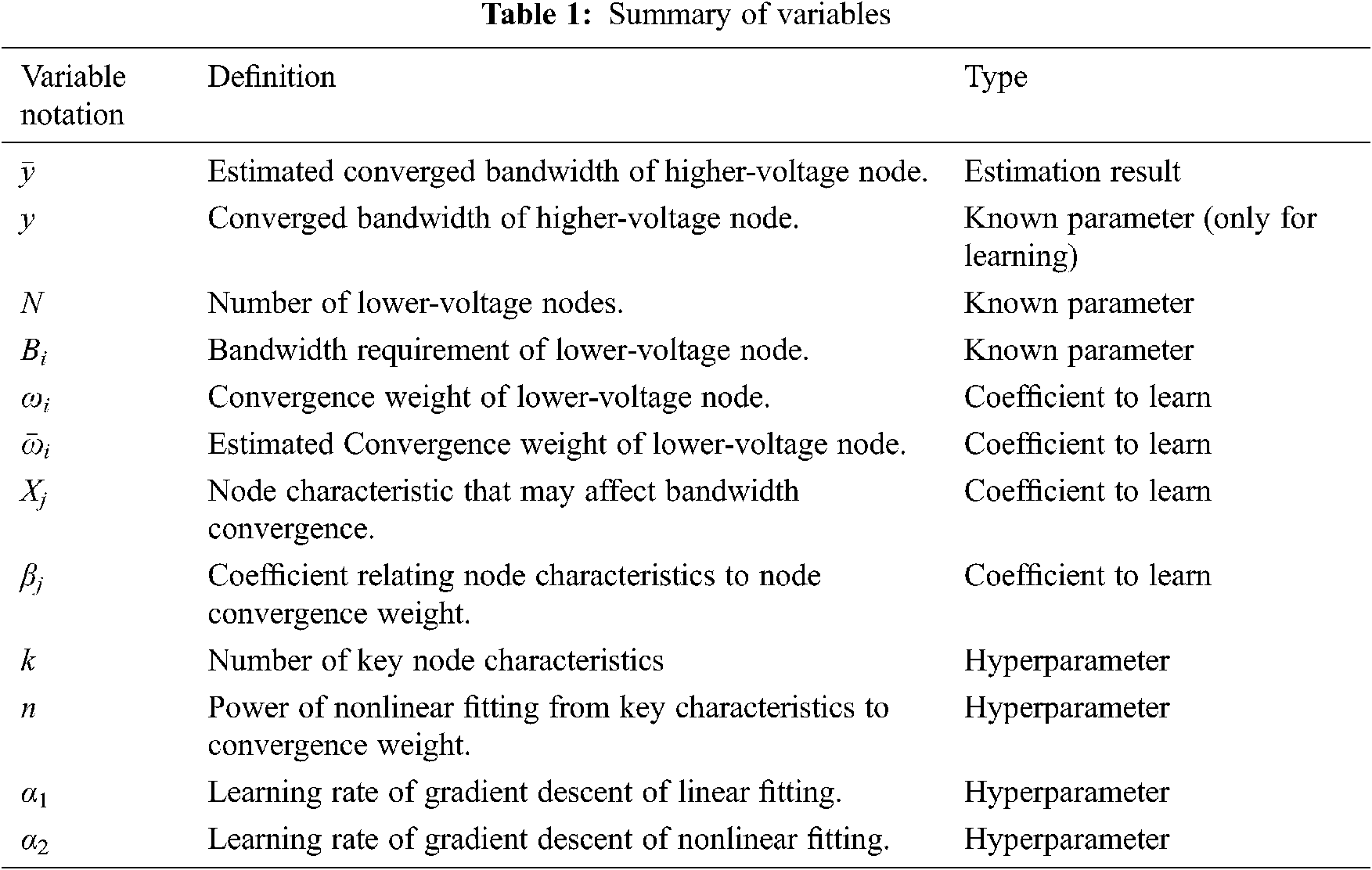
Based on the aforementioned features, we propose a fine-grained method for estimating bandwidth requirements of communication nodes in smart grid. We divide and study the characteristics of each node to obtain a more accurate bandwidth estimation method. Tab. 1 summarizes the variables used in this paper.

As shown by Fig. 2, our basic idea is using lower-voltage nodes’ bandwidth requirements (which are derived from application requirements) to estimate the bandwidth requirements of higher-voltage nodes, and then use these bandwidth estimations to further estimate the bandwidth requirements of even higher-voltage nodes, and eventually estimate the bandwidth requirements of dispatching centers.

Figure 2: Fine-grained bandwidth estimation method

Specifically, the bandwidth of an upper node (a higher-voltage node or a dispatching center) can be estimated as follows:

y¯=∑i=1Nwi⋅Bi,wi∈[0,1] (1)

where y¯ is the estimated converged bandwidth of the upper node, B1, B2, …, BN are the total bandwidth requirements of N lower nodes (i.e., data uploaded by even lower nodes plus data generated by the node itself), w1, w2, …, wN are the convergence weights of the N nodes (i.e., the ratio of data to upload).

The convergence weight wi of node i must lie in [0,1] because a lower-voltage node can never transmit data more than its own bandwidth. The value of wi can be derived from k characteristics of node i:

wi=∑j=1kβj⋅f(Xj)+βk+1⋅g(X1,X2…Xk) (2)

where X1, X2, …, Xk are node characteristics, f( ⋅ ) is a multinomial function of single characteristic, g( ⋅ ) is a multinomial function of multiple characteristics, βj and βk+1 are coefficients relating node characteristics to node convergence weight.

Eqs. (1) and (2) reveal the bandwidth convergence of lower-voltage nodes to higher-voltage nodes (and dispatching centers), and how such convergence is affected by multiple node characteristics. This way, we achieve fine-grained estimations corresponding to the differences among nodes.

Notably, we have not determined which node characteristics should be considered, and how these characteristics are related to node convergence weight. These two issues will be solved by multivariate nonlinear fitting in the next section.

5  Multivariate Nonlinear Fitting Scheme

In this section, we propose a multivariate nonlinear fitting scheme to relating node characteristics to node bandwidth. In other words, our scheme will learn all the undetermined coefficients in Eqs. (1) and (2) from measured node bandwidth and characteristics.

As Fig. 3 illustrates, our fitting scheme has three major steps. The first step is linear fitting, which takes converged bandwidth as target value to construct the loss function. Linear fitting uses the gradient descent method to derive convergence weight for each node. The second step is correlation coefficient calculation, which is using correlation coefficient to find key characteristics with more significant impacts on convergence weight across network. The last step is multivariate nonlinear fitting. This step reveals the nonlinear relationship among multiple characteristics and the convergence weight of each node, and therefore relates node characteristics to node bandwidth.

Figure 3: Multivariate nonlinear fitting scheme relating node characteristics to node bandwidth

5.1 Linear Learning

Here we utilize gradient descent to learn node convergence weight from real bandwidth data. In brief, we iteratively calculate the cost between the estimated bandwidth (which is derived from node convergence weight) and the actual bandwidth, and update convergence weight with gradient descent [40], until the cost becomes minimal.

First, we initialize node convergence weights as small positive numbers that are randomly generated within (0, 1), and substitute these weights and the known bandwidth requirements of lower nodes into Eq. (1) to derive the estimated bandwidth of the upper node y¯ .

Then we calculate the cost for gradient descent as follows:

cost=(y−y¯)2 (3)

where y is the actual bandwidth of the converged node.

The idea of gradient descent is to minimize cost by gradually adjusting node convergence weights. Specifically, the gradient of the cost function can be computed as:

∂cost∂wi=2×(y−y¯)×Bi (4)

where wi and Bi are the convergence weight and the bandwidth of the node i, respectively.

We gradually adjust the convergence weight of each node as follows:

wi←wi−α1×∂cost∂wi (5)

where α1 is the learning rate of gradient descent. Its value will be determined by experiments later.

Eqs. (4) and (5) will be executed iteratively until the cost function converges to its minimum. The obtained convergence weight wi essentially reflects the radio of node i’s bandwidth that converges to its upper node.

5.2 Correlation Coefficient Calculation

We use correlation coefficient calculation to decide which node characteristics (e.g., number or type of application) have more significant impacts on convergence weight. Only these key node characteristics will be concerned for bandwidth estimation. This is to simplify the acquirement process of node characteristics as well as the subsequent non-linear multivariate learning.

Specifically, for all N nodes, we calculate correlation coefficient between each candidate characteristic and the set of convergence weights as follows:

corr(w,Xj)=cov(w,Xj)var(w)⋅var(Xj) (6)

where w is the set of the convergence weights of all nodes (obtained in Section 5.1), Xj is the set of the values of a candidate characteristic for all nodes, cov(w, Xj) is the covariance of w and Xj, and var(w) and var(Xj) are the variance of w and Xj, respectively.

After calculating the correlation coeffecients for all candidate characteristics, we choose the key characteristics with higher correlation coeffecients for the non-linear multivariate learning in the next subsection. The number of key characteristics should be carefuly decided to balance between implemation complexity and bandwidth estimation accuracy. This will be further disccussed in Section 6.

5.3 Nonlinear Multivariate Fitting

At last, we exploit nonlinear multivariate fitting to reveal how a node’s convergence weight is affected by its characteristics. Here, “nonlinear” is to reflect the complexity of such relationship, and “multivariate” is to reflect the combined impacts of multiple node characteristics. Multivariate nonlinear fitting means using mathematical model to express the nonlinear relationship between different characteristics and the convergence weight.

Since we have derived the convergence weight in Section 5.1 and the key characteristics in Section 5.2, we only need to determine the rest unknown parameters in Eq. (2), namely, the multinomial functions f( ⋅ ) and g( ⋅ ), and the coefficients βj and βk+1. This is accomplished through fitting Eq. (2) to the convergence weight obtained in Eq. (5).

First, suppose that we have decided there are k key characteristics and the power of f( ⋅ ) is n (we will discuss how to derive them later). The nonlinear influence of each characteristic Xj on the convergence weight can be expressed by:

f(Xi)=a1Xi+a2Xi2+……+anXjn (7)

and the nonlinearly correlated influence of the k key characteristics on the convergence weight can be expressed by:

g(X1,X2…,Xk)=b(1,2)X1X2+b(1,3)X1X3…+b(1,2,…,k)X1X2…Xk (8)

where the coefficients a1, …, an, b(1,2), …, b(1,2,…,k) will be learned later. It is noteworthy that the complexity of g( ⋅ ) is o(2k), which is why we should keep the number of node characteristics k as small as possible.

Second, we substitute Eqs. (7) and (8) into Eq. (2) to express the fitted convergence weight w¯i for node i as follows:

w¯i=∑j=1kβj⋅f(Xj)+βk+1⋅g(X1,X2…Xk) (9)

Third, we compare the fitted convergence weight w¯i in Eq. (9) to the convergence weight wi derived by Eq. (5), i.e.,

loss=∑i=1n(wi−w¯i)2 (10)

Now we can learn the undetermined parameters via multivariate gradient descent [10]:

θ=θ←α2⋅∂loss∂θ (11)

where α2 is the learning rate, and its value will be determined by experiments later. θ represents multiple variables a1, …, an, b(1,2), …, b(1,2,…,k), β1, …, βk+1.

The above Eqs. (10) and (11) will be executed iteratively until the loss function Eq. (10) converges to its minimum. By repeating this process on all node convergence weights, the values of a1, …, an, b(1,2), …, b(1,2,…,k), β1, …, βk+1 are learned.

5.4 Determining Hyperparameters

Finally, we determine the hyperparameters that should be set before learning, namely, the learning rates α1 in Eq. (5) and α2 in Eq. (11), the number of the key node characteristics n, and the power of nonlinear fitting k in Eq. (7).

We begin with the learning rates α1 and α2. We initially set them to very small values, e.g., 10−8, and observe that whether the cost in Eq. (3) or the lost in Eq. (10) steadily decreases as we perform linear fitting in Eq. (4) or nonlinear fitting in Eq. (11), respectively. If the decrement is too slow, we gradually increase α1 or α2 to learn the unknown parameters more drastically. On the other hand, if the decrement is unstable, we gradually decrease α1 or α2 to learn more cautiously. We keep adjusting α1 and α2 until the decrement is stable and notable. The resulting α1 and α2 will be used for learning later.

Afterwards, we determine the number of the key node characteristics n, and the power of nonlinear fitting k. For practical considerations, we should set them as small as possible (otherwise, there are too many variables to learn in Eqs. (7) and (8)). Therefore, we gradually increase them from n = 1 and k = 1. For each pair of (n, k), we use Eq. (6) to find the k key node characteristics, use Eqs. (9)–(11) to derive the other unknown parameters in Eqs. (7) and (8), and use Eqs. (1) and (2) to obtain bandwidth estimations for all upper nodes. This increment process stops as the bandwidth estimation accuracy has become reasonably high and the accuracy increment has become marginal. The pair of (n, k) that has the highest bandwidth estimation accuracy will be used for learning later.

After determining the hyperparameters α1, α2, n, and k, we can learn all parameters’ values in Eqs. (1) and (2) from a present network with Eqs. (3)–(11). Then we can use Eqs. (1) and (2) to estimate the bandwidth requirements of new networks.

6  Simulation Results

We perform NS2 and TCL simulations to test our estimation method. Among them, NS2 is an open-source simulation platform for network technology. TCL is the script language on NS2.The simulated networks are based on a real-world regional smart grid in China. The network topologies are set as Figs. 4 and 6, and the applications are configured and deployed according to [1].

Figure 4: Network for learning estimation parameters

Figure 6: Network for estimating bandwidth

6.1 Learning from Present Network

We learn the estimation parameters from the network in Fig. 4. This network is based on the regional power grid of a moderate-sized city in China, which has 2 regional dispatching centers, 9 220 kV substations, and 1 110 kV substation. It represents a “present network” where the nodes’ bandwidth consumptions have been known. During learning, Z2 node is used for validating, and the rest nodes are used for fitting.

We first determine the linear learning rate α1 and the nonlinear learning rate α2. We increase α1 and α2 from 10−8 to 10−4, respectively, and find that the fitting costs of Eqs. (4) and (11) stably decrease only when α1 ≤ 10−6 and α2 ≤ 10−6. Since larger learning rates lead to quicker learning, we choose α1 = 10−6 and α2 = 10−6.

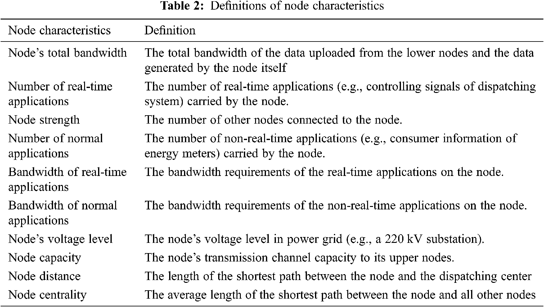
Next, we investigate 8 node characteristics that maybe related to convergence weight, as listed in Tab. 2.

We calculate correlation coefficient as Eq. (6) to find that there are k = 3 node characteristics closely related to convergence weight, which are: node’s total bandwidth > number of real-time applications > node strength.

We show 4 node characteristics with the highest correlation coefficient values in Tab. 3, which are node’s total bandwidth, number of real-time applications, node strength, and number of normal applications. It can be seen that while the first 3 characteristics have correlation coefficients larger than 0.6, the fourth characteristic (i.e., number of normal applications) drastically drops to 0.36. Such result indicates that number of normal applications (and the characteristics after it) has statistically ignorable impacts on convergence weight.

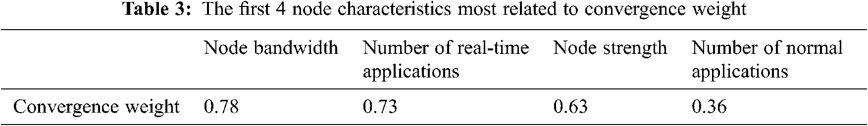
The above result is reasonable. Firstly, a node’s total bandwidth basically reflects how important it is for smart grid (as complex applications tend to be deployed in critical grid sites), which means that a node with higher bandwidth requirement often has proportionally more data to upload. Secondly, most real-time applications need to communicate with dispatching center, so a node with more real-time applications implies that it has more data to upload. Thirdly, a node with higher node strength means that it is connected by many other nodes, so it tends to have more data to upload. Later we will show that our estimation based on these three characteristics indeed achieves rather high accuracy.

Afterwards, we determine the power of Eq. (7), n. According to Eq. (9), the value of n directly affects the fitting performance from node characteristics to convergence weight. To demonstrate this, we draw the fitting curves relating the 3 node characteristics (for conciseness, we only show each node’s total bandwidth on the x-axis) to the 11 nodes’ convergence weights in Fig. 5. Observe that the fitting curve can barely match itself to all the points when n ≤ 2, which means that the relationship between the node characteristics and the convergence weight is too complicated for these values of n to capture. When n ≥ 3, the fitting curve is able to reach most of the points, and thereby the convergence weight is well related to the node characteristics.

Figure 5: The fitting curves relating node characteristics to convergence weight for different values of n. Note that Z2 is excluded here for it is used for validating (a) n = 1 (b) n = 2 (c) n = 3 (d) n = 4

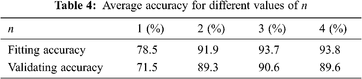
Nevertheless, according to machine learning theory, n being too large will lead to overfitting, that is, our method can achieve high accuracy during learning, but its accuracy will drop if it is applied to nodes excluded by learning process (i.e., Z2 in this case). This statement is verified by Tab. 4, where we compute the average bandwidth estimation accuracy across the network for different values of n. Observe that although the fitting accuracy keeps increasing as n grows, the validating accuracy for Z2 reaches the maximum at n = 3, and decreases as n becomes larger. This clearly indicates that overfitting occurs for n > 3. Combing this result with Fig. 5, we let n = 3.

Finally, with k = 3 and n = 3, we can further derive the values of a1, …, an, b(1,2), …, b(1,2,…,k), β1, …, βk+1. The deriving process and the final results are omitted here.

6.2 Estimating on New Network

Now we use the results in Section 6.1 to estimate the network bandwidth in Fig. 6. This network is based on a small city’s power grid, which has 1 regional dispatching centers, 1 220 kV substations, 5 110 kV substation, and 1 35 kV substation. This represents a “new network” where only applications’ bandwidth requirements are known. Note that the network is highly heterogeneous with 4 different types of nodes, which is difficult for bandwidth estimation.

We are mostly interested in the estimation accuracy of the dispatching center, because it is the most important node in smart grid’s control system, and its estimation accuracy basically depends on the estimation accuracies of all the other nodes. Tab. 5 compares our method with 3 recent works in [2,4,6], where t, a, and b mean that network topology, applications, and node’s total bandwidth are considered in estimation, respectively.

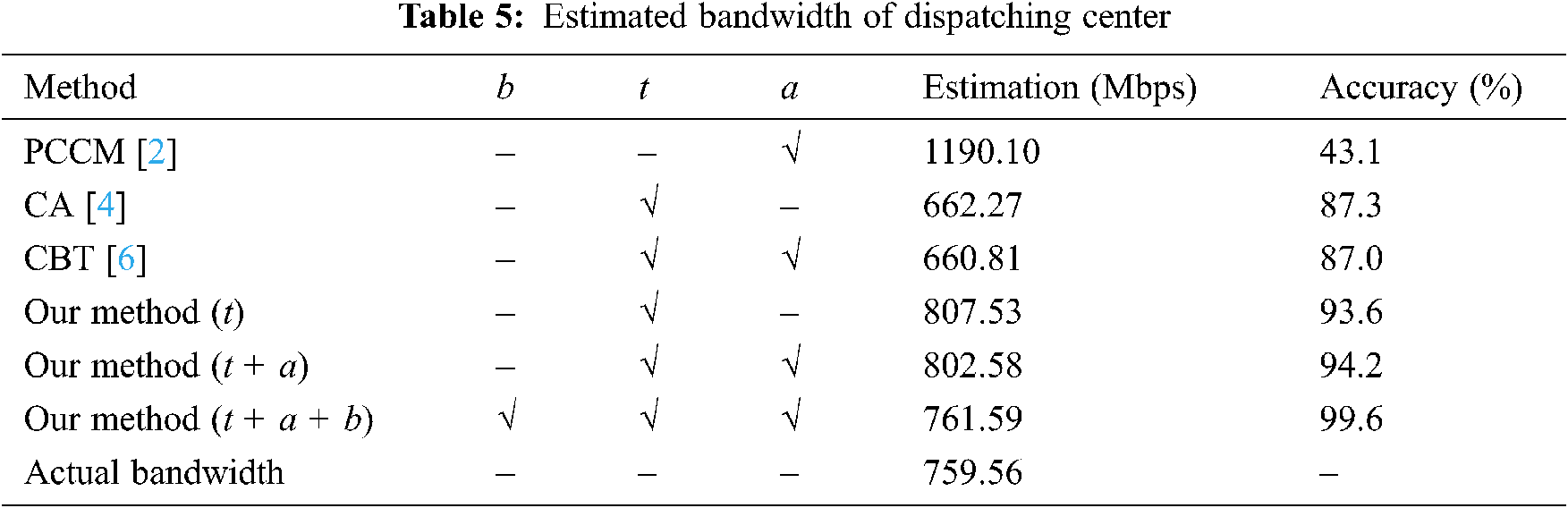
Observe that our method (t + a + b) is just slightly higher than the actual bandwidth requirement of 759.56 Mbps, which outperforms the alternative methods (PCCM [2], CA [4], and CBT [6]) by 12.6% to 56.5% higher accuracy. The major reason is that our method accomplishes finer-grained estimation via considering network topology (node strength), applications (number of real-time applications), and node bandwidth as key node characteristics (see Section 6.1). In contrast, the alternative methods only consider one or two of these characteristics, thus they can hardly differentiate the convergence impacts of different lower-voltage nodes on the dispatching center.

In fact, Tab. 5 also shows that our method achieves higher accuracy as it takes more characteristics into consideration, i.e., t < (t + a) < (t + a + b). Such result further proves that finer-grained estimation leads to higher accuracy.

We further investigate how the selection of node characteristics affects convergence weight learning, and eventually affects bandwidth estimation. This can be clearly illustrated by the ranking of learned convergence weights of different methods in Tab. 6.

By considering node strength (t), number of real-time applications (a), and node bandwidth (b), our method derives the same ranking as the actual network does. As the matter of fact, for the dispatching center (S7), the ranking of the convergence weights of all nodes should be: itself (S7), the nodes linked by lower-voltage nodes (S2, S6, and S4), the nodes without lower-voltage nodes (S0, S1, S3), and the lowest-voltage nodes (S5, S8). Our method’s fine-grained recognition of different nodes is the key to accurate bandwidth estimation.

On the other hand, because PCCM ignores network topology and node bandwidth, it cannot fully recognize the differences among various nodes to learn convergence weights in a heterogeneous network like Fig. 6. This explains why PCCM has rather low estimation accuracy in Tab. 5.

Both CA and CBT have considered topology for estimation, so they can roughly infer how the nodes converges the dispatching center, and hence make partially correct rankings in Tab. 6. However, note that both CA and CBT incorrectly rank S3 after S5 due to their neglection of node bandwidth. This explains their relatively low estimation accuracy in Tab. 5.

7  Conclusion

In this paper, we propose a novel fine-grained bandwidth estimation method for smart grid communication network. The method achieves fine-grained estimations through explicitly considering how bandwidth requirements of different nodes converges to upper nodes, and it exploits multivariate nonlinear learning to derive multiple convergence parameters from present network without needing human experience. Due to these two novelties, our method outperforms existing methods by up to 56.5% higher estimation accuracy. Through the comparison of different characteristics, we find that the fitting accuracy of the three characteristics selected in this paper is higher, which can reach 99.6%. In future, we will collect transmission data from other industrial Internet to train this model. So that this method can be applied to other Industrial Internets, such as the communication networks of railway or oil pipeline. Furthermore, we will study how to directly estimate bandwidth requirement and predict long-term development based on current network information using deep learning and big data technologies.

Funding Statement: This work was supported by Natural Science Foundation of China (Grant No.62071098); Sichuan Application and Basic Research Funds (Grant No. 2021YJ0313); Sichuan Science and Technology Program (Grant No. 2021YFG0307).

Conflicts of Interest: The authors declare that they have no conflicts of interest to report regarding the present study.

This work is licensed under a Creative Commons Attribution 4.0 International License, which permits unrestricted use, distribution, and reproduction in any medium, provided the original work is properly cited.