Soil Urea Analysis Using Mid-Infrared Spectroscopy and Machine Learning

J. Haritha; R. Valarmathi; M. Kalamani

doi:10.32604/iasc.2022.022547

1Department of Electronics and Instrumentation Engineering, Bannari Amman Institute of Technology, Erode, 638401, India
2Department of Electronics and Communication Engineering, Vel Tech Rangarajan Dr Sagunthala R & D Institute of Science, Chennai, 600062, India
3Department of Electronics and Communication Engineering, KPR Institute of Engineering and Technology, Coimbatore, 641048, India
*Corresponding Author: J. Haritha. Email: haritha.jeganathann@gmail.com
Received: 11 August 2021; Accepted: 12 October 2021

Abstract: Urea is the most common fertilizer used by the farmers. In this study, the variation of mid-infrared transmittance spectra with addition of urea in soil was studied for five different concentrations of urea. 150 gm of soil is taken and dried in a hot air oven for 5 h at 80°C and then samples are prepared by adding urea and water to it. The spectral signature of soil with urea is obtained by using an Infrared Spectrometer that reads the spectra in the mid infra-red region. The analysis is done using Partial Least Square Regression and Support Vector Machine algorithms by applying Savitzky Golay filter and Gaussian filter. The score plot, prediction and reference plots are used in the analysis using PLSR. RMSE and R-squared value are obtained from the analysis. It is evident that the detection accuracy was appropriate for Gaussian filter compared to Golay filter for both the PLSR and SVM models. The RMSE for PLSR is 0.8% and for SVM is 16%. The results show that Support vector machine model has higher accuracy compared to Partial least square regression model considering the prediction for which R square value is 0.99 with and without filters. SVM model gives better prediction without filters.

Keywords: Infrared spectroscopy; soil; partial least square regression; support vector machine

Soil is an important source of nutrients, minerals and several other constituents that is required for plant growth and for decomposing the dead matters. The essential macronutrients for plants present in the soil naturally are Nitrogen (N), Phosphorus (P) and Potassium (K). The NPK level in the soil will decide which plant is suitable for their land. NPK may be present in their form or different form i.e., the nitrogen may be in ammonia form. The nitrogen present in the soil may get evaporated. Several fertilisers are used to improve NPK content in soil. Soil nitrogen is an important component that enriches the plant growth. The most common fertilizer to improve the nitrogen content in soil is urea. The excess use of urea can also damage the crops. It is therefore essential to analyse the urea content in soil and thereby estimate the amount of nitrogen in soil. The standard methods are costly when a large number of samples is needed for analysis. Therefore, rapid and low-cost technique is needed for precision farming. Mid Infra-red (MIR) spectroscopy method shown to be fast, simple, convenient, accurate and able to analyse more nutrients at the same time.

Near Infra-red (NIR) spectroscopy is used to find chemical and physical properties of the samples which samples are measured using NIR spectroscopy. In this method 165 samples were collected from a particular area in different places, 135 spectra samples were used during analysis of nutrient content and calibration. They have used principle component analysis (PCA) and partial least square algorithm (PLS). This method is expensive when a high number of samples are used for testing [1–4]. In imaging spectroscopy, the main parameters discussed are soil erosion, deposition, soil genesis and formation, soil contamination, salinity, soil mapping and classification, soil swelling and soil water content [5]. Using the electrical properties of the plant tissues, it is easy to find the Nitrogen statues of plants [6]. The sensing methods are used to supervise soil carbon effectively, and it is critical to implementing best agronomic practices that require carbon sequestration and greenhouse gas (GHG) emission reduction [7]. The sensing will help to better articulate the carbon sufficient level will be known and it will fulfil the need of carbon in food, fibre, environmental and climate adaptation [8]. The impact of drying and sieving the soil samples while determining the total nitrogen, phosphorus and potassium contents in a soil sample, by using Vis-Near Infrared Spectroscopy and Mid-Infrared spectroscopy shows that the high prediction error can limit the applicability of spectroscopy to direct the use of the variable-rate application offer within the scope of precision farming [9]. The effect of two digestion methods like standard Kjeldahls and salicylic acid modification were analysed on plant nutrients [10]. For characterizing the mesenchymal stem cells growth this paper suggests using electrode based electrical impedance spectroscopy chips by eliminating the use of chemical marker [11]. The leaf epidermal chlorophyll and polyphenol content were measured by Dualex, SPAD and SPAD/Dualex ratio methods and compare the result. From the experiment result it shows that the SPAD/Dualex ratio and Dualex are the more hopeful method for Nitrogen measurement [12]. The method used for measuring Crop Nitrogen Status (CNS) were concentration tests of petiole sap nitrate and leaf chlorophyll then the final one is crop light reflectance test. It also covers most recent CNS assess methods [13].

The understanding of soil organic and moisture content is responsible for the plant growth and health. The ability of predicting these components using a Near Infrared Sensor was examined. The different pre-processing techniques to remove outliers were detailed. The Standard error technique was used to validate the NIR sensor prediction of organic matter and moisture level [14]. A partial least squares (PLS) model for determining the contamination level of zinc (Zn) and cadmium (Cd) in soil were proposed [15]. The comparison of the four methods like salicylic acid modification, combustion using LECO FP-428, phenyl acetate addition and NO3-N to NH4-N reduction with standard Kjeldahl nitrogen digestion method were done. The nitrogen content was measured on soil, water and body and plant tissue. This analysis helps to choose the correct method based on the requirement [16]. The three calibration methods like partial least squares regression (PLSR), principal component regression (PCR) and back propagation neural network (BPNN) were taken and analysed to estimate Sodium (Na), Potassium (K), Phosphorous (P) and Magnesium (Mg) content of soil [17]. The soil sample is collected from the ground and soil spectral data collected from the lab and satellite sensor [Remote sensing data]. By using the soil sample the attributes like sand, clay, were calculated by the laboratory analyses method. The multiple regression method is used to estimate the soil attributes. The estimated soil attribute from Remote Sensing data and calculated soil attributes from field soil samples were evaluated using R-squared (R2) value [18].

The canonical discriminant analysis, principal component analysis and depth of band analysis were done for examining an iron content and organic matter. From the analysis result it is clear that the spectral shape is affected by the iron and organic matter [19]. The N content calculated by the two wavelength [690 nm and 730 nm] ratio. And it also details the advantages of statistical methods by comparing it with reflectance-based measurements [20]. Soil water content is determined by developing the model called Soil Moisture Gaussian Model using Gaussian function [21]. The hyperspectral index of a single leaf is not that much sensitive to N content when the nitrogen fertilization is high. But the proposed method using a modified simple ratio of leaf positional difference is highly correlated to all levels of Nitrogen fertilization [22]. The soil properties are measured using visible and short wave near infrared spectroscopy and it is found that least square support vector machine outperformed the partial least square model [23]. Soil organic matter and pH is studied using vis-NIR spectra and it is found that extreme learning machines provide accurate results when used with genetic algorithm [24]. Soil total nitrogen content is studied using deep learning models [25]. The literature study shows that all the existing methods are laboratory based and consumes lot of time to study the soil major nutrients. Also, all the methods involve high cost analytical instruments for measurement and analysis. The proposed method is an approach to implement machine learning algorithm into a handheld spectrometer using the MIR (5.5 μm to 12.5 μm) data for identifying the soil nutrients more precisely and accurately. In this project work, the data is mainly analysed for the variation in urea content in soil as it is the most commonly used fertilizer to enrich the nitrogen fixation in soil. The entire analysis is done using Unscrambler (Evaluation version) tool.

The land is prepared (548 × 640 cm area) in an Agricultural plot, Bannari Amman Institute of Technology College, Sathyamangalam, and Tamilnadu. Soil samples were collected from the prepared plot. Soil samples were transferred to air tight plastic bags. By sieving process, grass, stones and other external objects were removed from the soil samples. Here the sieving is done using 2 mm sieve.

150 gm of soil is taken and dried in a hot air oven for 5 h at 80°C. It was split into 6 samples, each sample containing 20 gm of soil. Urea is added with each 20 gm soil as 0, 0.5, 1, 2, 3 and 4 gm respectively. Then, the soil sample is mixed with 10 ml of water and kept for one day is mixed with 25 ml of water and stirred. Next the mixed soil sample is filtered, and water sample collected in beaker. Then finally filtered with help of filter paper and collected in the sample tubes for MIR spectroscopy analysis.

Mid-infrared spectroscopy is a very essential and generally used sample analytical method. It detects the fundamental vibrations of minerals and organic matter, which have strong absorptions. MIR is used in chemical composition of materials. MIR spectroscopy is mostly used in the pharmaceutical industry because of high informational content of the spectra. The spectral range of the MIR spectroscopy is 400 cm−1– 4000 cm−1 (2500 – 25000 nm). Electromagnetic radiation is passed through the sample, the sample absorbs and reflects the radiation, with help of the absorption and reflection, the spectra is created. The resulting spectral signature shows how much energy was absorbed at each wavelength. It also responds to mineral composition and soil organic. The absorption reveals the molecular structure of the sample and quality of the sample. MIR is low cost, to detect the soil without chemical components and easy to work.

The Beer-Lambert law gives the relationship between the light attenuation and the same substance’s properties. The relationship can be exp

Attenuated Total Reflection (ATR) is a wave which is penetrating the electromagnetic field whose intensity decays quickly as it moves away from that source. The beam interacts and absorbs energy from the sample. So, the reflected wave’s intensity which reaches the detector is reduced. An Attenuated Total Reflection is the most essential technique used in laboratories for sampling, allowing for quick analysis of liquid and solid materials. MIR spectra are a powerful technique to identify the unknown chemicals. ATR generally allows little or no preparation of samples which greatly accelerates sample analysis. It allows the IR beam to penetrate into the sample in very thin path length and depth. It is useful for samples which are too thick to be examined during transmission and those which absorb radiation strongly.

Absorbance is a measure of the amount of light with a defined wavelength which prevents a given material from going through it. The transmittance is described as the ratio of the transmitted intensity over the light intensity.

In order to measure a sample in a spectrometer, a reference sample is required for performing computations. In the proposed method, the sample is analysed in the Mid Infra-red region of the spectrum. Here, water sample is used as reference as the soil samples are prepared using water. Once the sample is placed on the spectrometer, it starts scanning the sample and the intensity of the sample under test is recorded for the wavelength from 5.5 μm to 12.5 μm (wavenumber 1800 cm−1 to 800 cm−1) with a sample interval of 0.04 μm. Hence, for a single sample, 128 intensity data are recorded for the wavelength from 5.5 μm to 12.5 μm in Comma Separated Value (CSV) format and the readings can be visualised as a graph between intensity and wavelength on the interface software of the spectrometer. First, the water sample is to be analysed in MIR spectroscopy. Then the soil samples are intensity spectra is recorded as it is done for the water sample. Each soil samples are subject for recording 30 spectral data in order to train the model developed using Partial Least Square Regression (PLSR) and Support Vector Machine (SVM). This is the initial procedure for collecting the data. This process is repeated for the remaining five soil samples. Finally, 6 types of sample data are collected in six different folders. Each data folder contains 33 data sets, which contains 3 water samples data and 30 soil samples data. The folders’ names are indicated as Pure Soil, Soil Urea 0.5 gm, Soil Urea 1 gm, Soil Urea 2u gm, Soil Urea 3 gm, Soil Urea 4 gm. All folders are consolidated with the help of python program.

Partial least squares regression is a popular numerical method. The basic principle of PLSR is finding the correlation between the sample and variable. The sample data is plotted and decomposed into latent structure after several iterations. Then the T vector was found which shows most variation in sample data. The same plotting and decomposition were done for variable data also. The most variation in variables was represented by the U vector.

The plotting of u and t will give the relationship between variable and sample. The underlying model of PLSR is given as

Using the projection [U, T] and orthogonal matrices [P, Q] were able to construct the regression model between X and Y. The regression equation is given as

Support vector machine was used for multi class classification. The number of SVM models used for multi classification was equal to the number of classifications. The SVM model is given below

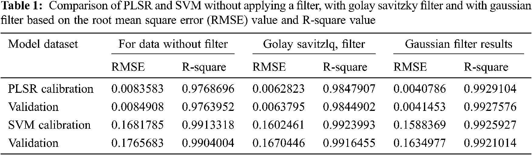
The soil divided into 6 parts and in each part, urea was mixed at different concentrations. The 6 soil samples were analysed using MIR spectroscopy. First the raw data was used to develop the PLSR and SVM model for soil classification based on urea content. Then the data was pre-processed using Savitzky-Golay filter (zero order) and Gaussian filter (window size 7). Again, the PLSR and SVM model was developed for pre-processed data. After that all the two models with and without filtered data were compared for finding the best method. All the spectral analysis, pre-processing and model evaluation techniques are done using the Unscrambler (Evaluation version) tool and is discussed in the following sections. It is observed that results show that Root Mean Square Error (RMSE) is very minimum using PLSR model compared to SVM model as indicated in Tab. 1. Though PLSR model has the RMSE value of 0.8% when compared to SVM model which has RMSE value of 16%, the prediction accuracy is decided by the R2 value. From Tab. 1 it is evident that SVM model gives better prediction compared to the PLSR model as its R2 value is 0.99.

The 6 types of soil samples with various urea concentration are analysed using the MIR spectroscopy. The spectra of standard urea solution using FTIR has peaks that can be observed in the range from 1500 cm−1 to 1800 cm−1 and from 3500 cm−1 to 3800 cm−1 [7]. The line graph plot for the entire raw spectroscopy data is shown in Fig. 1a. In this graph, the x-axis is the wavenumber in cm−1 of spectrum and y-axis represent the transmittance value in percentage. For classifying the different concentrations of urea in the soil spectra, spectrum data between wavenumber 1300 cm−1 and 1850 cm−1 as shown in Fig. 1b is taken for further analysis. From Fig. 1, it can be clearly observed that the variation in soil spectra for different concentrations of urea is seen at wavenumber 1560 cm−1.

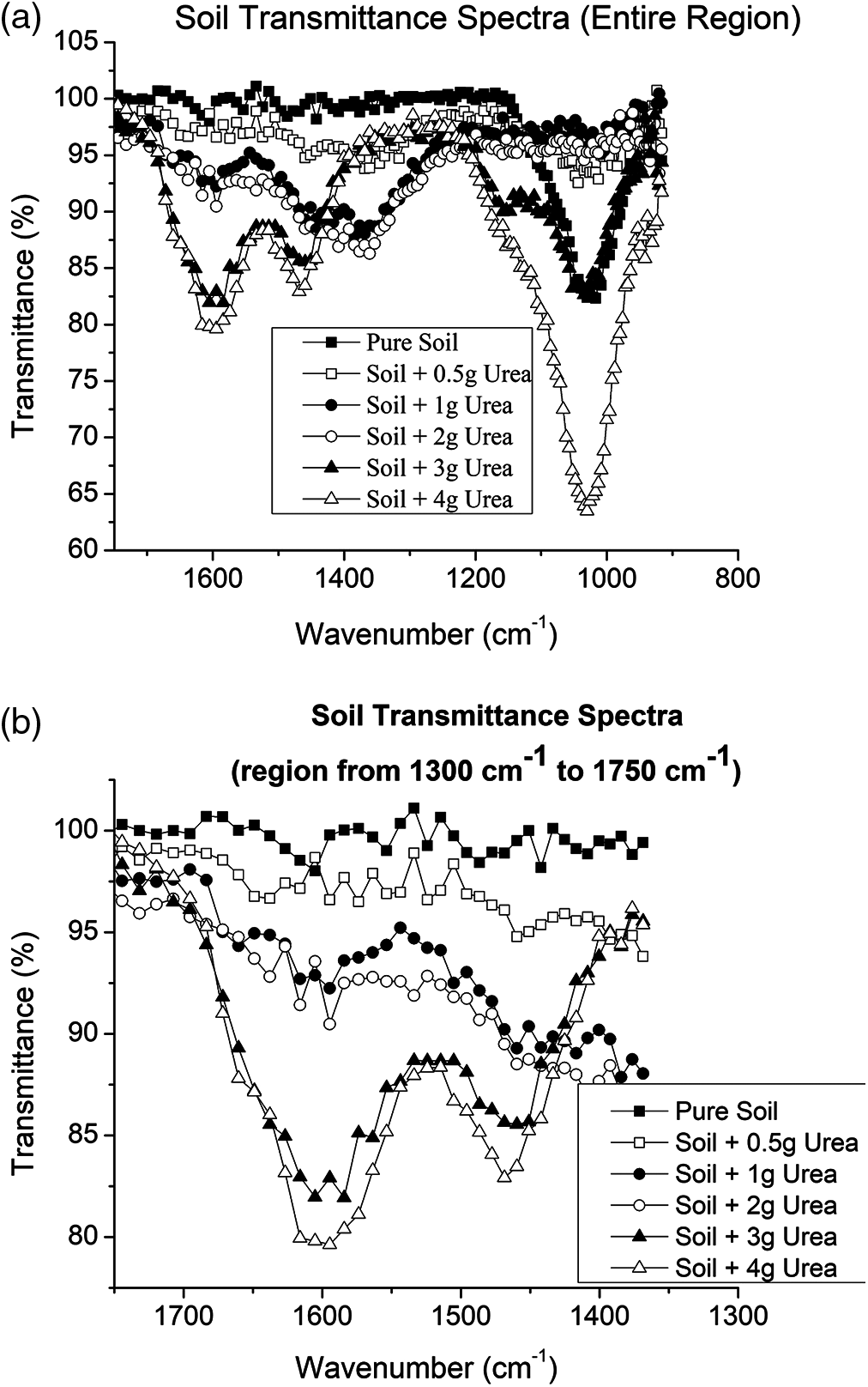
Figure 1: Soil urea transmittance spectra plotted using the recorded mid infrared spectrometer data. The recorded intensity is converted into transmittance and plotted against the wavenumber in cm−1 (a) entire spectra (b) spectra between wavenumber 1300 cm−1 and 1750 cm−1

The PLSR model was developed for the soil spectra dataset between wavenumber 1300 cm−1 and 1850 cm−1. For model valuation the score plot was used and it is shown in Fig. 2a. It shows the details of the classification of soil based on the projection of data. For finding the outliers the Hoteling’s T2 was used which is represented as an eclipse. The data at the outside of eclipse are considered as outliers. The factor 1 in the X-axis shows that 87% of X variation tells 87% of Y variation and similarly factor 2 gives the details of X and variation. These factor details are important for model evaluation.

Figure 2: PLSR evaluation plot for soil transmittance spectra without filter [for wavenumber between 1300 cm−1 and 1850 cm−1] (a) Score Plot - shows the details of the classification of soil based on the projection of data. (b) The predicted and reference sample of calibration and validation dataset

The predicted and reference sample of calibration and validation dataset were shown in Fig. 2b. It provides the slope and offset value of the regression equation used for calibration and validation model. Then for evaluating the designed model Root Mean Square Error and R-squared values were used.

The R-squared value i.e., the coefficient of determination is calculated using the formula

The Root Mean Square Error (RMSE) is the standard deviation of the residuals i.e., the prediction errors and is obtained by squaring the residuals, find the average of the squared residuals and finally taking the square root of the results. The RMSE shows how far the data points are closer to the regression line. It is given by

The spectrum data with wavelength 1300 cm−1 and 1850 cm−1 was taken and developed using SVM. The SVM classifies the urea content in soil based on the hyperplane. The number of hyperplanes depends on the number of samples needed to be classified. The classification of soil using SVM based on urea content is shown in the Fig. 3. The designed calibration and validation model were evaluated using Root Mean Square Error and R-squared values.

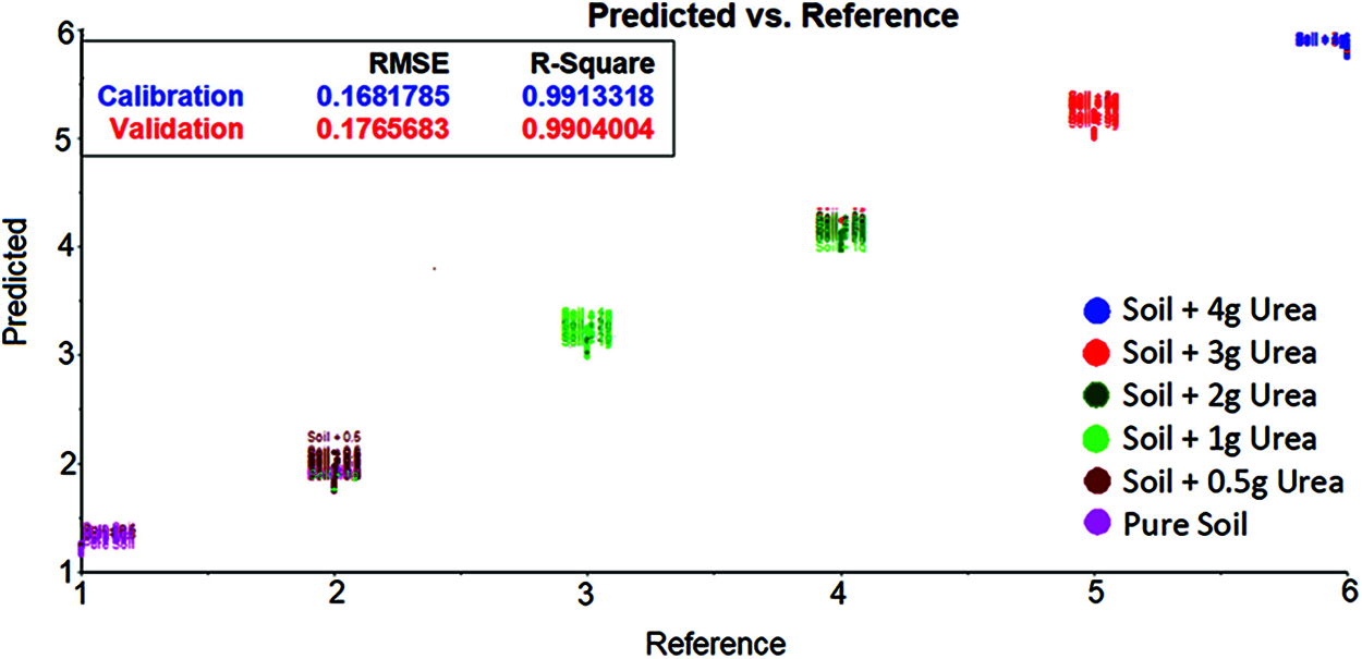
Figure 3: SVM evaluation plot for soil transmittance data without filter [between 1300 cm−1 and 1850 cm−1 wavenumber] shows the urea content in soil based on the hyperplane

3.3 Soil Spectral Analysis with Savitzky-Golay Filter Using Partial Least Square Regression

The Savitzky-Golay filter is applied to the spectrum data for smoothing the signal. It is used to reduce the presence of tiny noise signals. The concepts behind this filter are convolution and polynomial approximation. The polynomial coefficients are linear to the raw data values. If the smoothing window size is N*N and the polynomial order is k. The general filter equation for smoothing is

For fitting the polynomial in the raw data equation, the coefficient has to find by solving the least square

Because of linearity fitting to the data, the coefficient should be calculated independently. For that the unit vector replaces the f in the equation. Then the coefficient matrix converted as follows

The 1st coefficient was used to smooth the spectrum data. The other coefficients were used to compute derivatives. The Golay filtered data with wavenumber 1300 cm−1 and 1850 cm−1 after was considered for urea content classification. The PLSR model was developed using the new dataset. The same steps and plots discussed in 3.1 were used to evaluate the PLSR model. The evaluation plot of the developed PLSR model after applying Golay filter is shown in Fig. 4. The score plot displayed Fig. 4a shows that the 90% of X variation gives information about 90% of Y variation. It seems that when compared to no filter method, the Golay filter method gives more correlation between the samples and variables. This pre-processing technique gives acceptable Root Mean Square Error and R-squared values which is seen in the bottom of Fig. 4b.

Figure 4: PLSR evaluation plot for soil transmittance spectra with savitzky golay filter [for wavenumber between 1300 cm−1 and 1850 cm−1] (a) Score plot - shows the details of the classification of soil based on the projection of data. (b) The predicted and reference sample of calibration and validation dataset

3.4 Soil Spectral Analysis with Savitzky-Golay Filter Using Support Vector Machine

The spectrum data after applying Golay filter with wavelength 1300 cm−1 and 1850 cm−1 was taken and developed using SVM. The classification of soil based on urea content is shown in the Fig. 5. The same parameters as no filter were used to evaluate the model. By comparing the Golay filter and no filter result. It seems that the no filter gives good Root Mean Square Error and R-squared values.

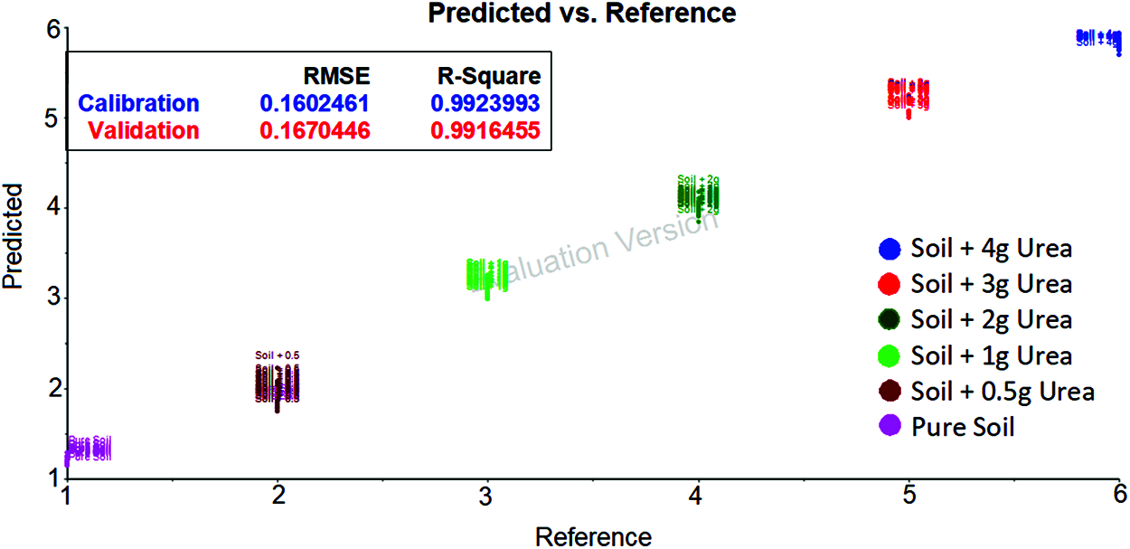
Figure 5: SVM evaluation plot for soil transmittance data with savitzky golay filter [between 1300 cm−1 and 1850 cm−1 wavenumber] shows the urea content in soil based on the hyperplane

3.5 Soil Spectral Analysis with Gaussian Filter Using Partial Least Square Regression

The Gaussian filter is based on 2-D convolution and it is used to smoothening the data by removing the noise. It is somewhat similar to the mean filter, but the kernel used in this filter varies. A Gaussian filter alters the input data by convolution with the help of Gaussian function. In 1D, the Gaussian function is given as

The Gaussian filter was applied to the raw spectrum data to smoothening the signal. After pre-processing by Gaussian filter the spectrum data with wavelength 1300 cm−1 and 1850 cm−1 was taken. The PLSR model was developed for this new dataset. The PLSR score plot of Gaussian filter data is shown in Fig. 6a which tells that the 91% of X variation gives information about 91% of Y variation. This filter data gives 1% extra correlation between the samples and variables than the Golay filter data. The bottom of the Fig. 6b shows the predicted and reference data plot and it clears that this type of filter gives better Root Mean Square Error and R-squared values compared to the Golay filter.

Figure 6: PLSR evaluation plot for soil transmittance spectra with gaussian filter [for wavenumber between 1300 cm−1 and 1850 cm−1] (a) Score plot - shows the details of the classification of soil based on the projection of data. (b) The predicted and reference sample of calibration and validation dataset

The spectrum data after applying Gaussian filter with wavelength 1300 cm−1 and 1850 cm−1 was taken and developed using SVM. The classification of soil based on urea content is shown in the Fig. 7. It can be observed that the predicted and reference are associated close to each other.

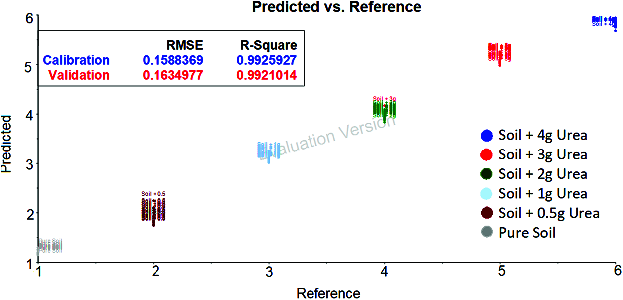
Figure 7: SVM evaluation plot for soil transmittance data with gaussian filter data [between 1300 cm−1 and 1850 cm−1 wavenumber] shows the urea content in soil based on the hyperplane

The Tab. 1 shows the comparison of the calibration and validation of PLSR and SVM model developed using data without filter, with Golay Savitzky filter data and with Gaussian filter data. From the Tab. 1 it clarifies that the SVM gives better R-squared values in all the cases compared to the PLSR method. Also, it can be observed that spectral analysis with Gaussian filter provides 99% accuracy which is the highest compared to the spectral data analysis without filter and with Golay Savitzky filter for both the methods. Since, SVM shows better performance with and without filter and hence it is proposed to use SVM compared to PLSR for implementation.

Soil urea detection based on Mid Infrared spectroscopy and machine learning has become more feasible but the performance of prediction is based on the algorithms implemented. The result of this work indicates that the pre-processing technique is much important for increasing the accuracy of soil urea detection. The best pre-processing technique is assessed by comparison. This comparison shows that the Gaussian filter is better than the Savitzky-Golay filter. RMSE is 0.8% for PLSR model and 0.16% for SVM model without filter and is further reduced when pre-processing is used with Golay and Gaussian filter. Though RMSE is very low for PLSR, R square value decides the prediction of results and the results shows that SVM has better R square values with and without filter. The R-squared parameters values shows that Support Vector Machine model has higher accuracy compared to Partial Least Square Regression model with a factor of 0.99. In future, a portable handheld device will be designed in by incorporating this model. This device definitely will revolutionize the agricultural field. The farmer can use this device for protecting their crops from excess and lack of urea content. It helps them to increase their productivity.

Acknowledgement: We would like to thank the Management, Bannari Amman Institute of Technology for providing support by providing the agricultural plot for this research and Robert Bosch, Bangalore for providing MIR spectrometer to measure the soil spectra for analysis.

Funding Statement: The authors received no specific funding for this study except for the soil samples collected from agriculture plot located at Bannari Amman Institute of Technology, Sathyamangalam, India and spectrometer instrument provided by Robert Bosch, R&D, Bangalore.

Conflicts of Interest: The authors declare that they have no conflicts of interest to report regarding the present study.

References

Y. He, M. Huang, A. García, A. Hernández and H. Song, “Prediction of soil macronutrients content using near-infrared spectroscopy,” Computers and Electronics in Agriculture, vol. 58, no. 2, pp. 144–153, 2007.
V. Bellon-Maurel, E. Fernandez-Ahumada, B. Palagos, J. -M. Roger and A. McBratney, “Critical review of chemometric indicators commonly used for assessing the quality of the prediction of soil attributes by NIR spectroscopy,” TrAC Trends in Analytical Chemistry, vol. 29, no. 9, pp. 1073–1081, 2010.
P. Nie, T. Dong, Y. He and F. Qu, “Detection of soil nitrogen using near infrared sensors based on soil pre-treatment and algorithms,” Sensors, vol. 17, no. 5, pp. 1–12, 2017.
D. Cozzolino and A. Moron, “Influence of soil particle size on the measurement of sodium by near-infrared reflectance spectroscopy,” Communication in Soil Science and Plant Analysis, vol. 41, no. 19, pp. 2330–2339, 2010.
E. Ben-Dor, S. Chabrillat, J. A. M. Demattê, G. R. Taylor, J. Hill et al., “Using imaging spectroscopy to study soil properties,” Remote Sensing of Environment, vol. 113, no. 1, pp. S38–S55, 2009.
R. F. Muñoz-Huerta, R. G. Guevara-Gonzalez, L. M. Contreras-Medina, I. Torres-Pacheco, J. Prado-Olivarez et al., “A review of methods for sensing the nitrogen status in plants: Advantages, disadvantages and recent advances,” Sensors, vol. 13, no. 8, pp. 10823–10843, 2013.
A. Raphael, V. Rossel and J. Bouma, “Soil sensing: A new paradigm for agriculture,” Agricultural Systems, vol. 148, pp. 71–74, 2016.
M. Manivannan and S. Rajendran, “Investigation of inhibitive action of urea- Zn2+ system in the corrosion control of carbon steel in sea water,” International Journal of Engineering Science and Technology (IJEST), vol. 3, no. 11, pp. 8048–8060, 2011.
A. N. Marcos Coutinho, O. Fernando de Alari, M. C. Márcia Ferreira and R. Lucas do Amaral, “Influence of soil sample preparation on the quantification of NPK content via spectroscopy,” Geoderma, vol. 338, pp. 401–409, 201
M. Amina and T. H. Flowers, “Evaluation of kjeldahl digestion method,” Journal of Research (Science), vol. 15, no. 2, pp. 159–179, 2004.
S. Cho and H. Thielecke, “Electrical characterization of human mesenchymal stem cell growth on microelectrode,” Microelectronic Engineering, vol. 85, no. 5, pp. 1272–1274, 2008.
S. Demotes-Mainard, R. Boumaza, S. Meyer and Z. G. Cerovic, “Indicators of nitrogen status for ornamental woody plants based on optical measurements of leaf epidermal polyphenol and chlorophyll contents,” Scientia Horticulturae, vol. 115, pp. 377–385, 2008.
J. P. Goffart, M. Olivier and M. Frankinet, “Potato crop nitrogen status assessment to improve N fertilization management and efficiency,” Potato Research, vol. 51, no. 3, pp. 355–383, 2008.
J. W. Hummel, K. A. Sudduth and S. E. Hollinger, “Soil moisture and organic matter prediction of surface and subsurface soils using an NIR soil sensor,” Computers and Electronics in Agriculture, vol. 32, pp. 149−165, 2001.
L. Kooistra, R. Wehrens, R. S. E. W. Leuven and L. M. C. Buydens, “Possibilities of visible–near-infrared spectroscopy for the assessment of soil contamination in river floodplains,” Analitica Chimica Acta, vol. 446, no. 1, pp. 97–105, 2001.
D. Lee, V. Nguyen and S. Littlefield, “Comparison of methods for determination of nitrogen levels in soil, plant and body tissues, and water,” Communication in Soil Science and Plant Analysis, vol. 27, no. 3, pp. 783–793, 1996.
A. M. Mouazen, B. Kuang, J. De Baerdemaeker and H. Ramon, “Comparison between principal component, partial least squares and back propagation neural network analyses for accuracy of measurement of selected soil properties with visible and near infrared spectroscopy,” Geoderma, vol. 158, no. 1, pp. 23–31, 2010.
M. R. Nanni and J. A. M. Dematte, “Spectral reflectance methodology in comparison to traditional soil analysis,” Soil Science Society of America Journal, vol. 70, no. 2, pp. 393–407, 2006.
A. Palacios-Orueta and S. L. Ustin, “Remote sensing of soil properties in the santa monica mountains: I. spectral analysis,” Remote Sensing of Environment, vol. 65, no. 2, pp. 170–183, 1998.
D. Thoren and U. Schmidhalter, “Nitrogen status and biomass determination of oilseed rape by laser-induced chlorophyll fluorescence,” European Journal of Agronomy, vol. 30, no. 3, pp. 238–242, 2009.
M. L. Whiting, L. Lin and S. L. Ustin, “Predicting water content using Gaussian model on soil spectra,” Remote Sensing of Environment, vol. 89, pp. 535–552, 2004.
Q. -f. Zhou, Z. -y. Liu and J. -f. Huang, “Detection of nitrogen-over fertilized rice plants with leaf positional difference in hyper spectral vegetation index,” Journal of Zhejiang University Science B, vol. 11, no. 3, pp. 465–470, 2010.
L. Xuemei and L. Jianshe, “Measurement of soil properties using visible and short wave-near infrared spectroscopy and multivariate calibration,” Measurement, vol. 46, no. 10, pp. 3808–3814, 2013.
M. Yang, D. Xu, D. S. Chen, H. Li and Z. Shi, “Evaluation of machine learning approaches to predict soil organic matter and pH using vis-nIR spectra,” Sensors, vol. 19, pp. 1–14, 2019.
Y. Wang, M. Li, R. Ji, M. Wang and L. Zheng, “Comparison of soil total nitrogen content prediction models based on vis-nIR spectroscopy,” Sensors, vol. 20, no. 24, pp. 1–20, 2020.

Intelligent Automation & Soft Computing DOI:10.32604/iasc.2022.022547
Article