Intelligent Automation & Soft Computing DOI:10.32604/iasc.2022.023510
Article

On NSGA-II and NSGA-III in Portfolio Management

Mahmoud Awad1, Mohamed Abouhawwash1,2,* and H. N. Agiza1

1Department of Mathematics, Faculty of Science, Mansoura University, Mansoura, 35516, Egypt
2Department of Computational Mathematics, Science, and Engineering (CMSE), Michigan State University, East Lansing, 48824, USA
*Corresponding Author: Mohamed Abouhawwash. Email: abouhaww@msu.edu
Received: 11 September 2021; Accepted: 27 October 2021

Abstract: To solve single and multi-objective optimization problems, evolutionary algorithms have been created. We use the non-dominated sorting genetic algorithm (NSGA-II) to find the Pareto front in a two-objective portfolio query, and its extended variant NSGA-III to find the Pareto front in a three-objective portfolio problem, in this article. Furthermore, in both portfolio problems, we quantify the Karush-Kuhn-Tucker Proximity Measure (KKTPM) for each generation to determine how far we are from the effective front and to provide knowledge about the Pareto optimal solution. In the portfolio problem, looking for the optimal set of stock or assets that maximizes the mean return and minimizes the risk factor. In our numerical results, we used the NSGA-II for the portfolio problem with two objective functions and find the Pareto front. After that, we use Karush-Kuhn-Tucker Proximity Measure and find that the minimum KKT error metric goes to zero with the first few generations, which means at least one solution converges to the efficient front within a few generations. The other portfolio problem consists of three objective functions used NSGA-III to find the Pareto front and we use Karush-Kuhn-Tucker Proximity Measure and find that The minimum KKT error metric goes to zero with the first few generations, which means at least one solution converges to the efficient front within a few generations. Also, the maximum KKTPM metric values don’t show any convergence until the last generation. Finally, NSGA-II is effective only for two objective functions, and NSGA-III is effective only for three objective functions.

Keywords: Genetic algorithm; NSGA-II; NSGA-III; Portfolio problem

1  Introduction

Genetic algorithms (GA) have been widely employed as optimization and search methods in a variety of problem domains [1,2], including industry [3], architecture [4], and research, over the past ten years [5,6]. Their strong applicability, global outlook, and ease of usage are the key explanations for their high success rate.

Genetic algorithms are the most common algorithms for solving many real-life applications. These algorithms are inspired by natural selection. Genetic algorithms are population search algorithms, which introduced the idea of survival of the best fitness function. Most of these algorithms incorporate the genetic operation to obtain the new chromosome (solution). The basic genetic operations are selection, crossover, and mutation [7].

In the past, the portfolio optimization problem was designed to find the configuration of assets that generated the maximum expected return which was the main criterion. However, this design changed in 1952, a new variable with the expected return was introduced by Harry Markowitz that called the risk of each portfolio. Thereafter, analysts began to incorporate a risk-return trade-off in their models [8]. Harry Markowitz doesn’t consider the real-world challenges as cardinality constraints, lower and upper bounds, substantial stock size, class constraint, round-lots constraint, computational power and time, pre-assignment constraint, and local-minima avoidance.

In this article, we solve the portfolio problem [9] using two genetic algorithms, NSGA-II and NSGA-III. The competing parameters in the portfolio dilemma are optimizing anticipated return and mitigating risk, also known as the Markowitz, mean-variance model [10].

1.1 Aim of the Study

This study aims to find the Pareto front for portfolio problems with two and three objective functions using the methods NSGA-II and NSGA-III which are simpler and easy to apply. Those methods can address portfolio optimization problems without simplification and with decent results in a fair amount of time, and it has a lot of practical applications. we obtained solutions for the portfolio models using NSGA-II and NSGA-III same as theoretical solutions.

1.2 Novelty and Contributions

The main contributions of this paper are as follows:

•   A genetic algorithm can be used to find the Pareto front for portfolio optimization problems which are the same as those found in other approaches.

•   A genetic algorithm can handle the portfolio optimization problems without simplification and with decent results in a fair amount of time.

•   The two cases studied were presented to prove the applicability of the genetic algorithm.

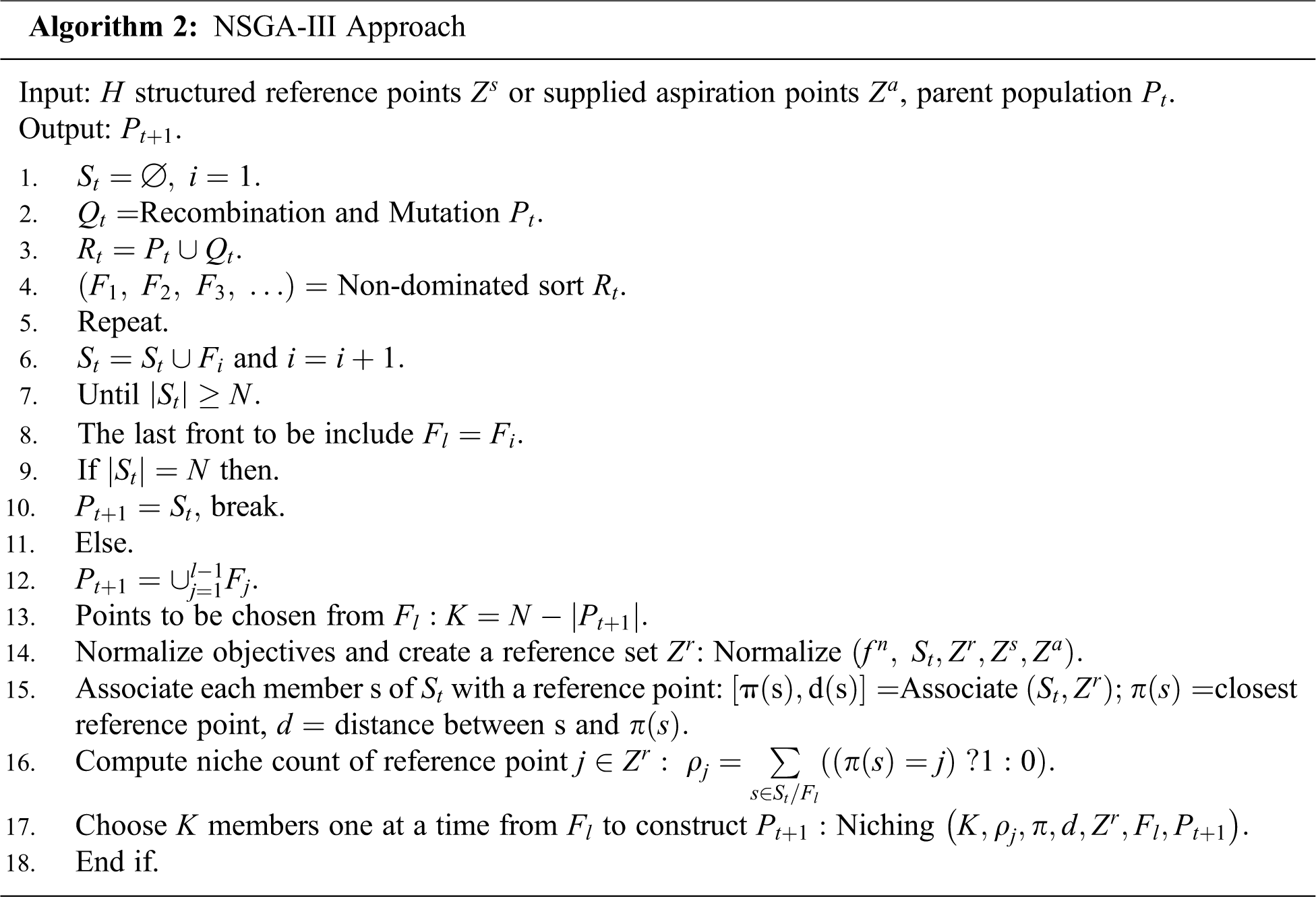
•   The framework of NSGA-II and NSGA-III are elaborated in algorithms 1 and algorithm 2.

1.3 Study Structure

In the following part of the article, we first give a literature review of NSGA-II, NSGA-III, and portfolio optimization problems in the second section. After that, we explain the concept of the NSGA-II method. The NSGA-III is discussed in the fourth section. The Karush-Kuhn-Tucker proximity measure (KKTPM) is analyzed in section five for multi-objective optimization problems [11,12]. In section six, evolutionary algorithms are used to solve a portfolio dilemma. Finally, in section seven, we bring the article to a close.

2  Literature Review

2.1 NSGA-II

There are many studies in NSGA-II. Deb et al. [13] have proposed NSGA-II which improves the iterative convergence rate while ensures population diversity by employing the fast non-dominated sorting approach. Kodali et al. [14] used NSGA-II to solve a problem that involves two objectives, four constraints, and ten decision variables of the grinding machining operation. Wang et al. [15] have used improved NSGA-II to solve multi-objective optimization of turbomachinery.

2.2 NSGA-III

There are some studies in NSGA-III. Deb and Jian [16] have proposed the first algorithm of NSGA-III to solve multi-objective optimization problems. Mkaouer et al. [17] are used NSGA-III to solve many-objective software remodularization. Zhu et al. [18] were studied an improved NSGA-III algorithm for feature selection used in intrusion detection. Yi et al. [19] were studied the behavior of crossover operators in NSGA-III for large-scale optimization problems.

2.3 Portfolio Problem

Markowitz [20] was proposed the portfolio problem, that it is looking for the expected mean-return is maximized (profit), and the risk is minimized. The factor in measuring risk is the variance of the portfolio return; the smaller the variance lower will be the risk. Michaud [21] has found that mean-variance theory has some limitations because asset volatility is required for constructing the model, and determining an asset’s future volatility is challenging in practice. Momentum investment is a well-known quantitative investment strategy. Hong and Stein [22] show that this strategy, the momentum effect is used to reveal the price stickiness of stocks over a certain period; this information is then used to predict price trends and make investment decisions.

3  NSGA-II or Elitist Non-Dominated Sorting GA

The NSGA-II protocols [23] is the most used EMO procedure for finding multiple Pareto-optimal solutions in a multi-objective optimization problem, and it has the following features:

It employs three principles: 1. an apparent diversity-preserving mechanism; 2. an elitist principle; and 3. non-dominated alternatives are stressed.

Consider a community of size N , with parent and offspring populations Pt and Qt . Making Rt=Pt∪Qt by combining offspring and parent populations in the first process. Rt should be non-dominated sorted to distinguish various fronts Fi,i=1,2,…, etc. Set a new population Pt+1=∅ and a counter i=1 before |Pt+1|+|Fi|<N is reached. Pt+1=Pt+1∪Fi and i=i+1 are the steps to take. Then use the crowding-sort (Fi,<C) protocol to get the most distributed (N−|Pt+1|) solutions by sorting the crowding distance values in the sort from Fi to Pt+1 . To build an offspring population Qt+1 from Pt+1 , use the crowded tournament array, crossover, and mutation operators.

Now we demonstrate a crowded tournament collection operator. The crowded comparison operator (<C) performs a comparison between two solutions and returns the tournament's winning answer. It is assumed that every solution i has two characteristics. The community has a local crowding distance (di) and a non-domination rating ri .

Definition: If all of the above assumptions are true, the crowded tournament selection operator [24] compares two solutions (solution i and another solution j ), and solution i wins the tournament. If ri<rj , it implies the solution i has a higher ranking. If ri=rj and di>dj , the solutions are of equal level, but solution i has a shorter crowding distance than solution j .

Crowding gap; To find the estimation density of solutions around a given solution i in the community, one takes the average distance between the two solutions on each side of solution i through each of the objectives. This di serves as the cuboid's estimated diameter, which is calculated by using the cuboid's nearest neighbors as vertices, a process known as crowding time. For each point in the set F , calculate the crowding distance as follows (crowding type (Fi,<C) : First and foremost, First, set di=0 for each i in the set. l=|F| equals the number of solutions in F. Find the ordered indices vector Im= sort (fm,>) for each objective function m=1,2,…,M , or sort in the collection in the worst order of fm . dI1m=dIlm=∞ or assign a significant gap to the boundary solutions for m=1,2,…,M , and all other solutions j=2 to (l−1) , assign:

dIjm=dIjm+fm(Ij+1m)−fm(Ij−1m)fmmax−fmmin (1)

The lowest and highest objective function values are denoted by I1 and Il , respectively. Algorithm 1, for generation t of NSGA-II procedure [25].

4  An Evolutionary Many-objective Optimization Algorithm Using Reference Point Based Non-Dominated Sorting Approach (NSGA-III)

NSGA-III begins [26] with a random population of N members and a series of widely spaced M -dimensional reference points H distributed over a unit hyper-plane with standard vector ones covering the entire R+M field. The hyper-plane (HP) is set up in such a way that it intersects all of the objective axes at the same time. The technique of Das and Dennis [27] is used to position H=(M+p−1p) reference points on the HP with (p+1) points through any boundary. They choose the population size N to be the smallest multiplied by four greater than H , with the assumption that one population member would be obtained for all reference points.

The following procedures are carried out at descent t . Following the precept of non-dominated sorting, all of the population Pt is sorted into different non-domination levels, close to how it is done in NSGA-II. The children's population Qt is generated by using standard mutation and recombination operators on the Pt population. Since only one population member is expected to be examined for any reference point, each selection procedure in NSGA-III is unnecessary, as every selection operator would allow competition to be established between different reference points. After that, a combined population Rt=Pt∪Qt is formed. Then, starting from the first non-dominated front, points are selected for Pt+1 one by one until no entire solutions from a full front can be used. This restriction is also common in the NSGA-II. Assume that there is a final front that can't be fully selected as FL . Only a few solutions from FL that choose to be selected from Pt+1 use a niche-preserving operator, which we'll look at later. To begin, any population unit of Pt+1 and FL is normalized using the current population distribution, resulting in similar values for all reference points and objective vectors. The shortest perpendicular distance (d()) of each population unit with a reference line generated by connecting a supplied reference point with the origin is then used to correlate each component of Pt+1 and FL with a specific reference point. Then, using reference points in Pt+1 , a cautious (NS) niching technique is used to pick certain FL components that are associated with the minimum. The (NS) niching strategy ensures that a population factor is selected for each of the provided reference points [28]. A population variable that is compared with an unrepresented comparison or an under-represented point is quickly outperformed. With a constant tension to ensure non-dominated individuals, all phase is predicted to produce one population variable that correlates with any supplied reference point near the (POF) Pareto-optimal front, assuming that the genetic difference operators (mutation and recombination) will deliver specific solutions. Algorithm 2 summarizes the algorithm, which uses widely spaced comparison points to ensure a well-distributed series of trade-off points at the end. Algorithm 2, Generation t of NSGA-III procedure:

5  Karush-Kuhn-Tucker Proximity Measure (KKTPM) for Multi-Objective Optimization

For a n -variable, M -objective optimization problem with J inequality constraints:

Subjecttogj(X)≤0,j=1,2,…,J, (2)

the Karush-Kuhn-Tucker optimality [29] conditions for Eq. (2) are given as follows:

∑m=1M⁡um∇fm(Xk)+∑j=1J⁡uj∇gj(Xk)=0, (3)

gj(Xk)≤0,j=1,2,…,J, (4)

ujgj(Xk)≤0,j=1,2,…,J, (5)

uj≥0,j=1,2,…,J, (6)

um≥0,m=1,2,…,M,andu≠0. (7)

The um multipliers are not negative, but at least one of them cannot be empty. For the j -th inequality constraint, the parameter uj is called Lagrange multiplier, and it is not even negative. A KKT point is a solution Xk that meets all of the above criteria. The inequality constraints gJ+2i−1(X)=xi(L)−xi≤0 and gJ+2i(X)=xi−xi(U)≤0 can be used to break inconstant the form xi(L)≤xi≤xi(U) . There are some J+2n inequality limits for the previous issue of whether there are whole n pairs with particular inconstant boundaries.

The authentic analysis generated an output scalarization feature (ASF) for a given repeated (solution) Xk [29]. A matter of optimization:

Subjecttogj(X)≤0,j=1,2,…,J. (8)

The reference point Z∈RM was believed as a utopian point and the weight vector W∈RM is computed for Xk as views:

wi=fi(Xk)−zi(∑m=1M⁡(fm(Xk)−zm)2)1/2. (9)

Thereafter, the KKTPM calculation process advanced for single-objective optimization problems to the ASF showed previously. So that the ASF formulation produce the objective function not differentiable, a smooth transformation of the ASF (a performance scalarization function) problem was made firstly by inserting slack variables xn+1 and reconstructing the initial problem as views:

Subjecttofi(X)−ziwik−xn+1≤0,i=1,2,…,M (10)

At this moment, the KKTPM optimization problem for the previous single-objective problem for y=(X;xn+1) can be written as follows:

∑j=1M+J⁡ujGj(y)≥−ϵk, (11)

The added term in the objective function permits a penalty correlated with the violation of the complementary slackness condition. The restrictions Gj(y) are given below:

Gj(y)=fj(X)−zjwjk−xn+1≤0,j=1,2,…,M, (12)

GM+j(y)=gj(X)≤0,j=1,2,…,J. (13)

The optimal objective value ϵk∗ to the above problem corresponds to the exact KKTPM. It is observed that for feasible solutions ϵk∗≤1 , hence the exact KKTPM was defined as follows:

Exact KKTPM

(Xk)={ϵk∗,feasibleXk,1+∑j=1J⁡gj(Xk)2,otherwise. (14)

6  Results Section

In this section, we will solve a portfolio problem in special cases using NSGA-II in the first model and NSGA-III in the second model. After that, we will show figures for each model. But, one must know the main portfolio problem. The portfolio is a set of assets or securities ( x1,x2,…,xn ) chosen to minimize the risk and maximize the expected return. The risk is measure by the variance. The problem can be written as following [30]:

To illustrate the mechanism of the evolutionary algorithms and KKT proximity measure using an evolutionary multi-objective (EMO) algorithm, we thought of three and two-objective Portfolio problems. NSGA-II is used to solve two objective problems, while NSGA-III is used to solve three objective problems. We use the SBX recombination operator [31,32] with pc=0.9 and ηc=30 in every problem, as well as the polynomial mutation operator [33,34] with pm=1/n (where n is the number of variables) and ηm=20 in every problem. In discussions about personal models, other criteria are listed.

6.1 Model-I for Portfolio Problem

Consider the three-security problems with expected returns vector and covariance matrix [35] given by:

(r1,r2,r3)=(0.062,0.146,0.128) and

Let X=(x1,x2,x3)T , where x1,x2,x3 are the proportions of an asset invested in the following model-I and model-II. So model-I is [19,20]

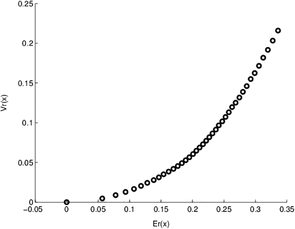
Figure 1: Pareto optimal points for model- I objective functions

Fig. 1 shows the non-dominated points for model-I. In this figure, NSGA-II runs 200 generations with 100 population sizes. The obtained solutions exactly equal the previously exact obtained solutions. One advantage of applying genetic algorithms is that we obtain many solutions in a single run. Also, Fig. 2 represents the relation between generation number and KKT proximity measure. As shown from the figures, the KKT metric reduces with increasing the number of generations.

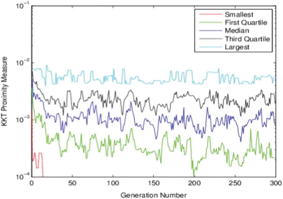
Figure 2: KKT Proximity measure vs. generation number for Model-I using NSGA-II

6.2 Model-Il for Portfolio Problem [31]:

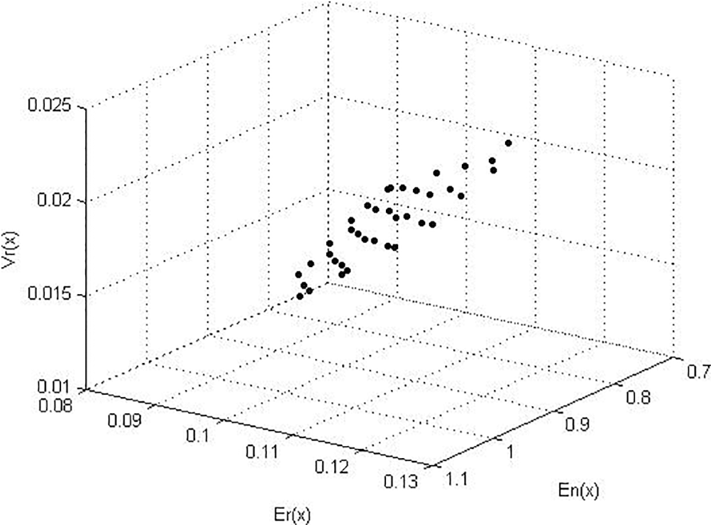
Figure 3: Pareto optimal points for model- II objective functions

Fig. 3 shows the non-dominated points for model-II obtained by the NSGA-III algorithm. In this figure, NSGA-III runs 300 generations with 100 population sizes. The obtained solutions for this model by the proposed algorithm equal previously published results for this model. In Fig. 4, the relation between generation number and the KKT proximity measure is introduced. As shown from the figures, the KKT metric reduces with increasing the number of generations.

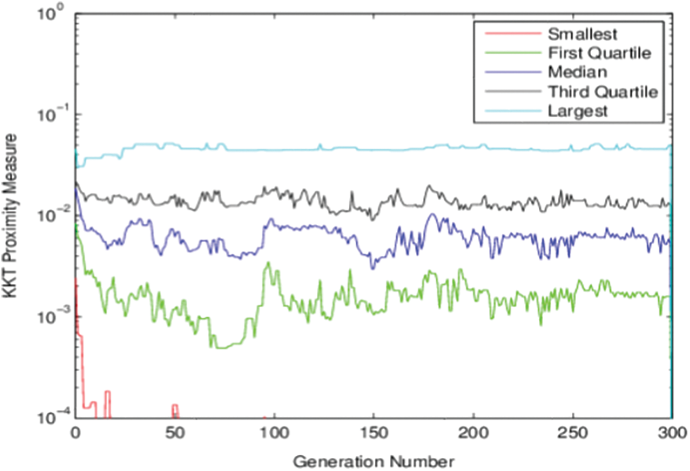
Figure 4: KKT Proximity measure vs. generation number for Model-II using NSGA-III

The minimum KKT error metric goes to zero with the first few generations, which means at least one solution converges to the efficient front within a few generations. Also, the maximum KKTPM metric values don’t show any convergence until the last generation.

7  Conclusion

The solutions found in genetic algorithms are the same as those found in other approaches, and they are as effective. The genetic algorithm, on the other hand, is simpler and easier to apply. A genetic algorithm can address portfolio optimization problems without simplification and with decent results in a fair amount of time, and it has a lot of practical applications. NSGA-II and NSGA-III are used to address portfolio problems in models I and II. We measure the smallest, first quartile, median, third quartile, and highest KKTPM values as a function of generation, and the figure shows that KKTPM values decrease with generation. The obtained solutions for the portfolio models using the genetic algorithms same as theoretical solutions. NSGA-II is effective only for two objective functions, and NSGA-III is effective only for three objective functions. NSGA-II can be solving real-life optimization problems with two objective functions, and NSGA-III can be solving real-life optimization problems with three objective functions. In the future direction of this work, we will extend the proposed algorithms with more real-life applications with many objective functions.

Funding Statement: The authors received no specific funding for this study.

Conflicts of Interest: The authors declare that no conflicts of interest occurred regarding the publication of the paper.

This work is licensed under a Creative Commons Attribution 4.0 International License, which permits unrestricted use, distribution, and reproduction in any medium, provided the original work is properly cited.