DOI:10.32604/iasc.2022.024264
| Intelligent Automation & Soft Computing DOI:10.32604/iasc.2022.024264 | |
| Article |
Sustainable Waste Collection Vehicle Routing Problem for COVID-19
1PSG Institute of Technology and Applied Research, Coimbatore, 641062, India
2PSG College of Technology, Coimbatore, 641004, India
*Corresponding Author: G. Niranjani. Email: niragopal@gmail.com
Received: 11 October 2021; Accepted: 12 November 2021
Abstract: COVID-19 pandemic has imposed many threats. One among them is the accumulation of waste in hospitals. Waste should be disposed regularly and safely using sustainable methods. Sustainability is self development with preservation of society and its resources. The main objective of this research is to achieve sustainability in waste collection by minimizing the cost factor. Minimization of sustainable-cost involves minimization of three sub-components – total travel-cost representing economical component, total emission-cost representing environmental component and total driver-allowance-cost representing social component. Most papers under waste collection implement Tabu search algorithm and fail to consider the environmental and social aspects involved. We propose a mathematical model, a novel algorithm called grouping algorithm, a combination of Nearest Neighbor algorithm and Simulated Annealing algorithm to achieve sustainable transportation in waste collection during pandemics. All these algorithms are run on Solomon’s and Gehring and Homberger’s benchmark dataset. The sustainable-cost obtained from the output routes of the proposed grouping algorithm is found to perform effectively for all the instances with minimized solution. The results are verified using computational techniques such as Integrated Ranking and Relative Percentage Deviation and statistical techniques such as Descriptive Statistics.
Keywords: Sustainable objective; grouping algorithm; nearest neighbor algorithm; simulated annealing algorithm
Waste materials, obtained from the hospitals, should be properly collected and effectively disposed. The recent pandemic conditions have further emphasized on timely transportation of waste materials such that they do not spread the disease further. The Vehicle Routing Problem (VRP) is a classical Combinatorial Optimization Problem that has many applications such as transportation of hazardous material [1], pharmaceutical distribution [2], food, raw material distribution, school bus routing [3] and scheduling. In this paper, we consider transportation of waste materials from hospitals to various disposal sites based on the type of waste using VRP.
There are many variants in VRP [4] depending on the application and the type of problem to be solved. This study deals with a Single Depot, Heterogeneous Vehicle Routing Problem with Time Windows (SD-HVRPTW).
This study focuses on minimization of distance and sustainable feature for VRPTW. The sustainability is captured by means of summing up the economic, environmental and the social factors. Each factor is calculated as a measure of cost–total travel-cost (Economic), total emission-cost (Environmental) and total Driver-allowance-cost (Social).
The solution approaches to solve VRPTW are classified as exact, greedy heuristics and Meta heuristics. A mathematical model based on [5] is formulated to solve to problem. This study proposes a new algorithm called the grouping algorithm which is used to group locations that are near to each other. This helps in disposal of waste with minimum cost. This algorithm can be combined with the existing greedy heuristic algorithm: Nearest Neighbor Heuristic that considers nearest location as the first point (NNH) and the single point meta-heuristic algorithm, Simulated Annealing. All these algorithms are executed on benchmark datasets. To differentiate the working of algorithms on different sizes of datasets, 56 instances of 100 locations–Solomon’s dataset [6] and 60 instances of 1000 locations–Gehring and Homberger’s dataset [7] are considered.
The performance of these algorithms is evaluated based on computational and statistical measures. For computational performance, the concepts of Integrated Ranking and Relative Percentage Deviation are considered and the statistical inference is done by means of Descriptive Statistics through which the algorithm that produces the minimized solution is identified.
This paper presents the closely related literature review on the waste collection problem in Section 2. Section 3 presents features and the mathematical model of VRPTW being used. Section 4 discusses the details on the proposed grouping algorithm with Nearest Neighbor and the Simulated Annealing algorithm. In Section 5, the performance evaluations of the proposed algorithms are discussed.
The waste collection is a separate category in the study of Vehicle Routing Problem with Time Windows stated by Beltrami et al. [8]. There are many solutions available for Vehicle Routing Problem as it is a NP-Hard problem [9]. The various algorithms used in waste collection transportation model under literature study are listed in Tab. 1.
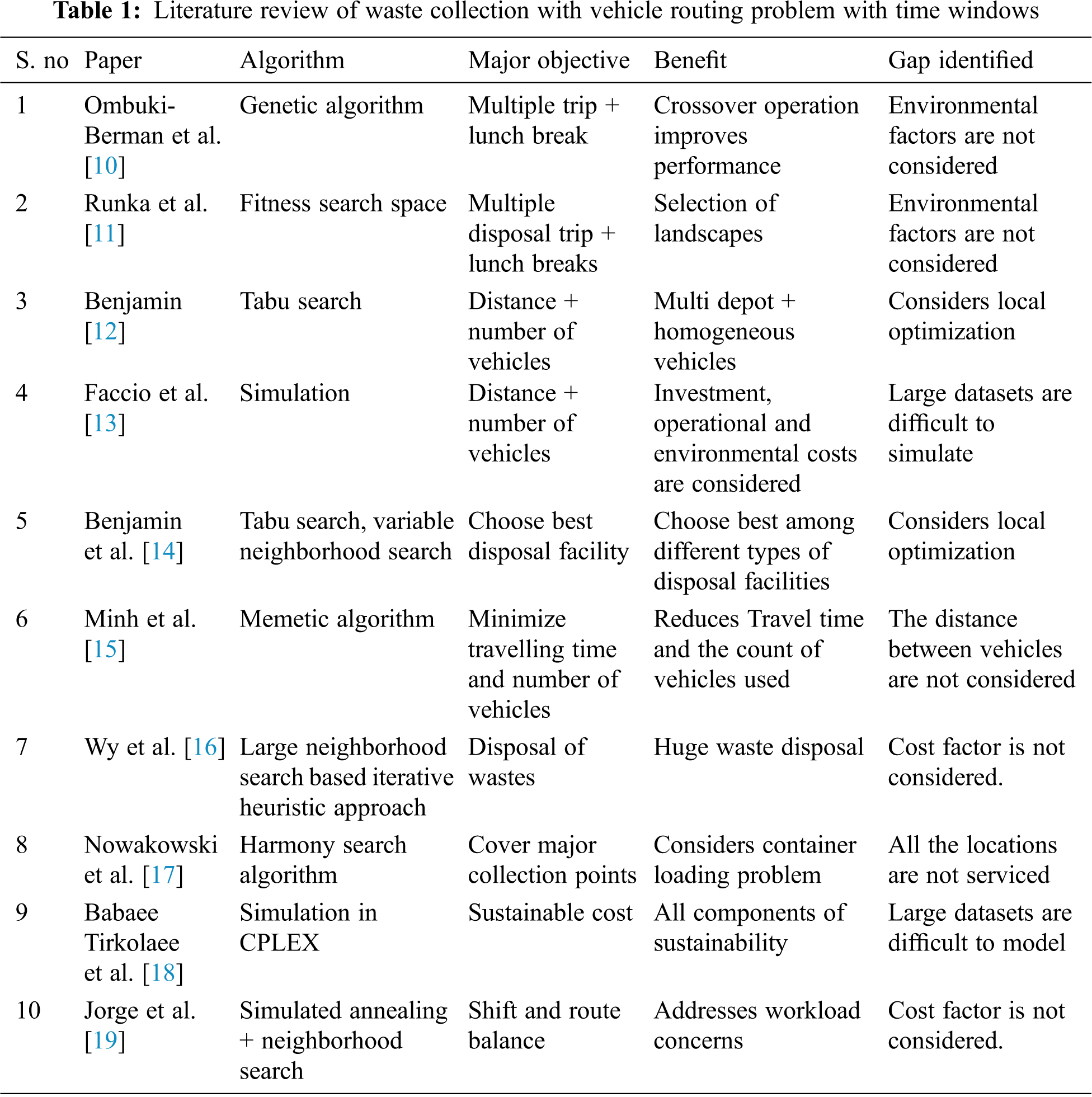
From Tab. 1, it is inferred that servicing most of the locations is also considered as a main objective in some papers. Other major objectives include–travelling time, route balance, cost factors, lunch break for drivers, distance. The algorithms in the literature [13] are limited to servicing only a few locations and end in local optimization.
This study services all the locations even if the problem size is high. Global optimization is addressed to obtain minimized cost. The proposed algorithm works well with scalable data.
3 The Proposed System for Waste Collection During Pandemic
The waste is collected from a single hospital (depot) and is transported to different disposal sites. The number of locations for disposing specific wastes is denoted by n and different types of vehicles by m. Each and every vehicle should start and end at the hospital. Each of these locations should be visited by one of the vehicles. Each vehicle visits a few locations depending on the capacity constraint and the time windows constraint specified. All the ‘n’ locations should be visited but all ‘m’ vehicles need not be used.
Each location including the hospital is defined by the following parameters:
• Customer-number (including hospital as location with number as ‘0’),
• x co-ordinate and y co-ordinate,
• Demand
• Start-time, End-time (denoted as Time Window) and Service-time.
Each vehicle includes the following features:
• Vehicle-number,
• Capacity,
• Mileage per unit of the fuel,
• Total-running-km,
• Age of the vehicle (in months),
• Emission-rate (in g/km), and
• Driver allowance for unit km.
These characteristics vary for each vehicle; and hence the problem comes under the category of heterogeneous fleet of vehicles [20]. The block diagram of the problem is presented in Fig. 1.

Figure 1: Block diagram of waste collection pandemic model
3.1 Proposed Mathematical Model for Sustainable SD-HVRPTW
The mathematical model generates the best solution for the waste collection pandemic model. The mathematical model is used to obtain the minimized cost when the number of vehicles and locations are limited. When the number of locations and the vehicles increase, the time for obtaining the cost increases exponentially. The sets and indices, Parameters, Variables and the MILP model are presented below:
Sets and Indices:
L – Set of Locations distributed around. L = {0, 1, …, m} where ‘0’ represents the hospital.
V – Set of Vehicles. V = {1, 2, …, n}
Parameters for location:
dij – Distance (Euclidean distance) between location ‘i’ and location ‘j’.
starti – Start time for location ‘i’
endi – Start time for location ‘i’
servicei – Time taken to dump waste in location ‘i’
Ai – Arrival time for location ‘i’
Parameters for vehicle:
capacityk – Capacity of vehicle k
ERk-Emission rate (grams per kilometer) for vehicle k
DAk-Driver-allowance rate (Rs. per liter) for vehicle k. It is an extra allowance that is notionally paid to the driver based on the pollution emitted and the distance travelled by the vehicle.
Distk-Distance travelled by vehicle k
DACk-Driver allowance cost for vehicle k
General parameters:
CP-Carbon pricing (a constant, penalty that is assumed to be imposed on vehicles based on the emission-rate and the distance travelled by the vehicle)
FC-Fuel cost (a constant, Rs. 70/-per liter)
TTC – Total travel-cost
TEC-Total emission-cost
TDAC-Total Driver-allowance-cost
Variable:
Objective function:
Subject to
Objective function
(1) This equation represents the Sustainable-cost.
(2) This equation is used to calculate the distance travelled by each vehicle which is the sum of Euclidean distance between consecutive locations serviced by the same vehicle.
The various constraints are represented as follows:
(3) For any vehicle, movement from one location to itself is not possible, except the hospital.
(4) All vehicles must start from the hospital.
(5) All vehicles must end at the hospital.
(6) To ensure that every vehicle starts only once from the hospital i.e., there are no multiple travels.
(7) All locations must be visited.
(8) The sum of demands of the locations visited by a vehicle does not exceed its capacity.
(9) Flow conservation Eqs. (10)–(12) These equations are used to ensure that the arrival time of a vehicle for a location must be greater than its start-time, less than its end-time and the arrival time of the next location processed by the same vehicle must be greater than the arrival time of previous location.
4 Proposed Algorithm for SD-HVRPTW
There are many algorithms [21–23] available for Vehicle Routing Problem with Time Windows. The grouping algorithm presented in 4.1 proposes heuristic solution for waste collection during pandemics.
The grouping algorithm is presented in the Fig. 2. In this algorithm, we take each and every location and group it with the other location which has the least distance among all the locations present in the dataset. They represent a group and are stored in a separate file. This file is accessed during the execution of other greedy heuristic and meta-heuristic algorithm to allocate locations to vehicles. When a single vehicle services all the locations present in a group, the distance factor is greatly reduced which subsequently leads to the minimization of sustainable-cost.

Figure 2: Flowchart for grouping algorithm
4.2 Proposed Grouping Nearest Neighbor Algorithm (G-NNH)
The pseudo code for the proposed G-NNH algorithm is given in Fig. 3. The Nearest Neighbor algorithm was proposed by Solomon [24]. It is also used in last mile deliveries [25]. In the NNH algorithm, for every vehicle, one location is selected based on the distance from the hospital and added to the route. Consequent locations are added to the same route which has the minimal distance from the last location serviced by the vehicle. The process is repeated until all the locations are serviced [26].

Figure 3: Grouping-Nearest Neighbor Heuristic (G-NNH) algorithm
In G-NNH algorithm, when a location is serviced by a particular vehicle, the other location belonging to group of the original location will also be serviced by the same vehicle. This leads to the reduction of distance travelled by all the vehicles and subsequently, the sustainable-cost.
4.3 Proposed Grouping Simulated Annealing (G-SA) Algorithm
Even though there are many meta-heuristic algorithms like Variable Neighborhood Search [27], we are using Simulated Annealing algorithm introduced by Kirkpatrick et al. [28] which is a single point meta-heuristic approach. Simulated Annealing algorithm is used for complex problems and is used to achieve global optimization instead of local optimization [29]. In this study, solution obtained from NNH and G-NNH is given one at a time as initial solution to the proposed SA and its variant-G-SA, respectively. The pseudo code of the proposed variant of SA is presented in Fig. 4.

Figure 4: Pseudo code for G-SA
The Simulated Annealing algorithm (SA) takes the output route from NNH algorithm as the initial input. A swap operation is carried out between locations of two different locations. After swap, if the objective value is minimized, the swapped route becomes the new solution. The same process is repeated based on the parameters.
In the proposed G-SA, the input is the output route obtained from G-NNH. For the swap operation, in addition to the location, the other locations that belong to a particular group are also swapped. The terminologies in Fig. 4 are as follows:
• Current-solution first refers to the output route obtained from G-NNH.
• Swap (ri, cm, group(cm), rj, cn, group (cn)) exchanges location ‘cm’ and group location of ‘cm’ from route ‘ri’ to location ‘cn’ and its group location from route ‘rj’ and vice-versa.
• N(S) indicates the feasible Neighborhood solution
• New-sus-cost denotes the sustainable-cost of solution after swapping.
Based on the analysis and the simulation output done on the dataset C1-10-1 for the parameters mentioned in [30–33], the following values are set for G-SA based on [33] for faster convergence:
• Initial Temperature (T0): 100
• Number of iterations (Max_no_of_Iteration): 300
• Cooling-factor (alpha): 0.9
• Final Temperature (TF): 0.001
The Nearest Neighbor algorithm selects the nearest location from the list of available locations and adds them to the route. This leads to increase in time for calculating routes and the possibility of two nearest locations being serviced by two different vehicles. Adding grouping algorithm greatly reduces these two disadvantages. Similarly, in the simulated annealing when locations between two different routes are swapped, their corresponding neighbors are also swapped decreasing the distances travelled by the corresponding vehicles.
To understand the performance and to evaluate the algorithms performance, a series of computational experiments are conducted. For those experiments, we need (i) Parameters, and (ii) Performance measures.
In this study, the distance, total travel-cost, total emission-cost, total driver-allowance-cost, sustainable-cost obtained from the NNH, G-NNH, SA, G-SA algorithms are considered for evaluation.
The empirical performance measure – Integrated Rank and Relative Performance Deviation (RPD) are used to assess the performance of algorithms. In addition, we consider the statistical measure–Descriptive Statistics. The performance measure considered is as follows:
Integrated RANK (IRANK): IRANK was introduced by Mathirajan et al. [34]. The formula used to calculate the IRANK is given in Eq. (13). It ensures the consistency of performance across all the instances for all the algorithms considered.
where
IRANK (A): Integrated RANK for Algorithm ‘A’
A: Algorithm, I: Rank
N(I, A): Number of times the solution of the algorithm ‘A’ is in RANK ‘I’ over 56 or 60 or 116 instances for benchmark datasets separately.
MaxRank: Maximum rank possible [This is equal to number of algorithms]
Relative Percentage Deviation (RPD): This is one of the standard performance measures for best case analysis given by Rardin et al. [35]. The formulae to compute relative percentage deviation with respect to the Estimated Optimal Solution (EOS) is given in Eq. (14).
where
SOA: Value obtained pertaining to corresponding algorithm for each of the instance.
EOS: Smallest value obtained among the 4 algorithms for each instance. If number of algorithms > = 7, EOS = 0.63*n + 1.
From the value of RPD, ARPD (Average RPD) and MRPD (Maximum RPD) is calculated for each of the instance using the Eqs. (15) and (16) respectively.
All the algorithms are implemented in C Programming on a computer: Intel® Core™ i5-4590 CPU @ 3.30 GHz with RAM: 4.00 GB.
Two types of benchmark datasets are considered:
• 56 instances of 100 location Solomon’s benchmark dataset
• 60 instances of 1000 location Gehring and Homberger’s benchmark dataset
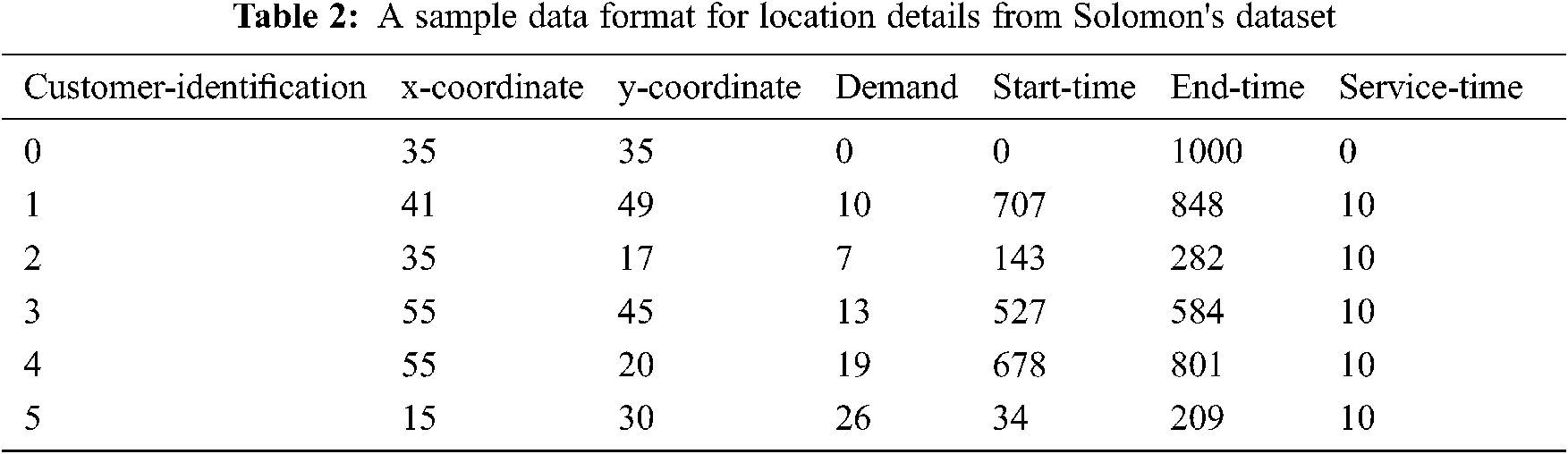
A sample data of customers is presented in Tab. 2. These benchmark datasets are chosen because they have been used in many papers available in literature from 1987 to 2021 to represent different applications of Vehicle Routing Problem [36].
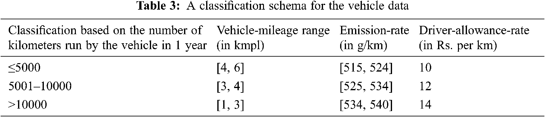
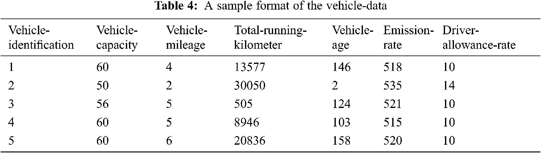
The data for the vehicles are generated as the benchmark instances are designed only for homogeneous vehicles and our problem considers a heterogeneous fleet of vehicles. The characteristics of the vehicle are generated based on the classification scheme in Tab. 3 and the sample is presented in Tab. 4. The capacity of the vehicles is 50, 56 and 60 (capacity of normal buses and vans on Indian roads) with a probability of 0.2, 0.3 and 0.5. A total of 800 vehicles are generated to accommodate 1000 locations.
Both the Greedy algorithms – NNH and G-NNH are evaluated using IRANK as in Tab. 5 and their mean, median are compared in Tab. 6.

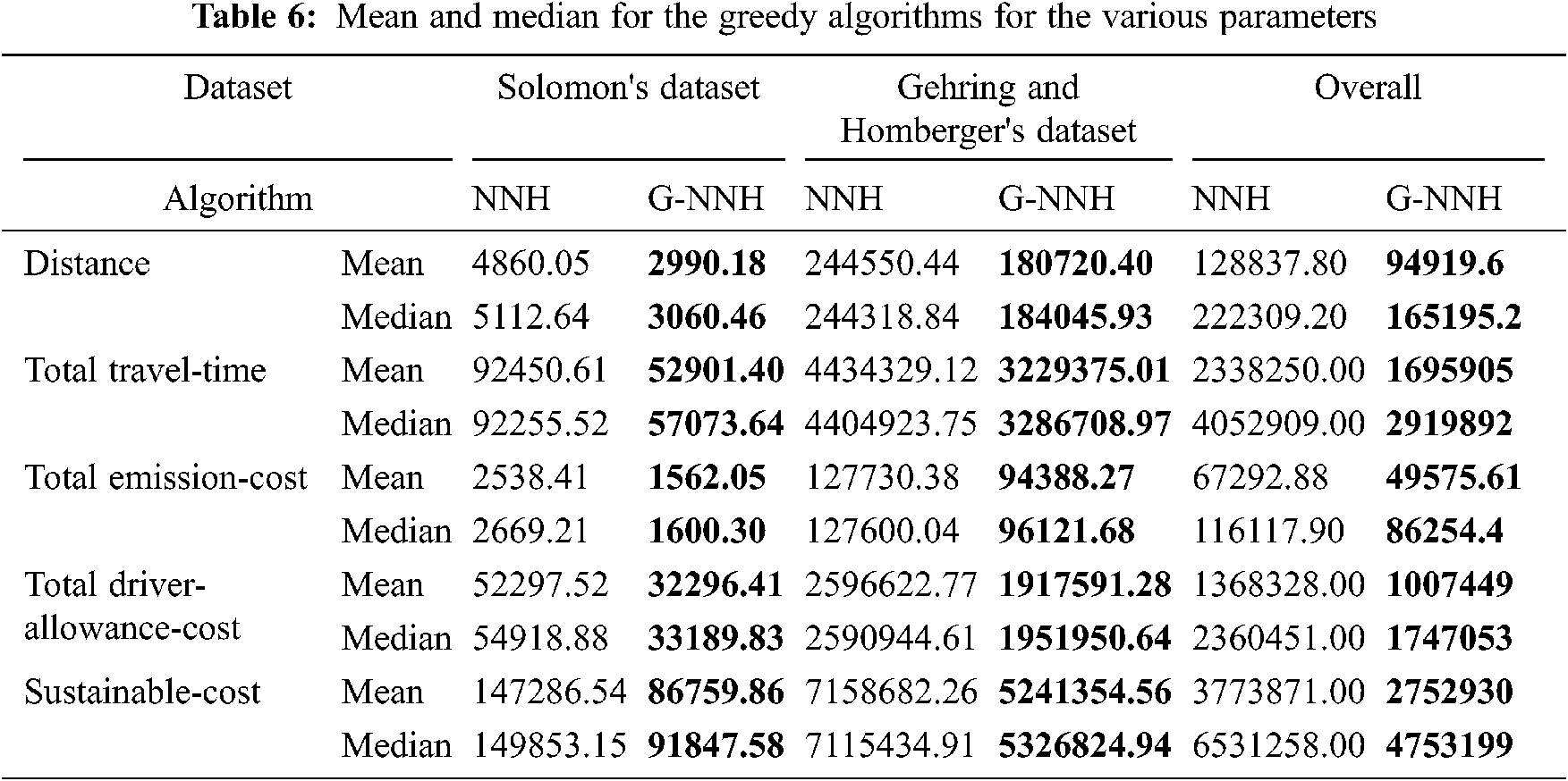
Inference: In Tab. 5, the values of Integrated RANK for all the parameters are presented. Integrated Rank is a measure that is used to check the consistency of a parameter across different kinds of instances. The ranking for Grouping-NNH is 1 which leads to the minimized value obtained. From Tab. 6, even the mean and median values are lower for all the parameters irrespective of the datasets. It further insists that the G-NNH algorithm gives 26% more efficient minimized solution than NNH for distance, 28% for total travel-cost, 26% for total emission-cost and total driver-allowance-cost and 27% for sustainable-cost.
The simulated annealing algorithm and the corresponding grouping variant are measured using Integrated Rank in the Tab. 7 and their mean and median are compared and presented in the Tab. 8.


Inference: Based on Tab. 7, the values of Integrated RANK for all the parameters are the least for Grouping-SA which leads to the minimized value obtained. From Tab. 8, the mean and median values indicate the corresponding values obtained in all the instances. Their values are lower for all the parameters irrespective of the number of locations in each instance. Based on this Tab. 8, the mean of G-SA algorithm are 26% more efficient in terms of distance, 27% in total travel-cost, 26% in total emission-cost and total driver-allowance-cost and 26% for sustainable-cost than SA algorithm for all the instances.
The comparison of all the four algorithms – NNH, G-NNH, SA, and G-SA in terms of Average Relative Percentage Deviation and Maximum Relative Percentage Deviation using Eqs. (15) and (16) are shown in Tab. 9 and the mean and median comparisons are presented in Fig. 5.


Figure 5: Comparison of mean and median obtained from NNH, G-NNH, SA, G-SA algorithms for different parameters, (a) Distance, (b) Total Travel-cost, (c) Total Emission-cost, (d) Total Driver Allowance cost, (e) Sustainable cost
Average Relative Percentage Deviation is the average value of RPD obtained from all the instances. The RPD considers the least value of the sustainable cost as the Estimated Optimal Solution as the number of algorithms considered is less than 7. MRPD is the maximum value obtained in all the instances for all the parameters. From Tab. 9, even though the ARPD and MRPD seem closer to each other, the single point variant of the meta-heuristic algorithm–G-SA produces the least value in all the three types of datasets. This means that the least sustainable-cost obtained from the G-NNH algorithm is further minimized by the Grouping variant SA. From the Fig. 5a represents the mean and median for total distance, Fig. 5b represents for total travel-cost, Fig. 5c represents for total emission-cost, Fig. 5d for total driver-allowance-cost and Fig. 5e for sustainable-cost. For all the parameters, the new algorithm–Grouping, when combined with Simulated Annealing algorithm gives the least value for all the benchmark instances. In terms of efficiency, for distance, G-SA is 26.42%, 0.13%, 25.73% more efficient than NNH, G-NNH and SA algorithms respectively. For total travel-cost, G-SA is 27.76%, 0.40%, 26.72% more efficient, for total emission-cost, 26.43%, 0.14% and 25.73%, for total driver-allowance-cost, 26.51%, 0.19% and 25.76%, and for sustainable cost, 27.29%, 0.32% and 26.35% more efficient than NNH, G-NNH and SA algorithms respectively.
Pandemic has a significant influence on us both financially and physically. The economic component is important in addition to disposing waste timely and efficiently by preserving the environment and taking care of co-workers. The proposed novel algorithm has greatly reduced the distance travelled by the vehicles, total travel-cost, total emission-cost, total driver-allowance-cost and hence, sustainable cost. The Grouping algorithm combined with Simulated Annealing algorithm helps to reduce the parameters involved to a great extent irrespective of the number of waste disposal sites available.
The scope of this study can be further improved by inserting the concept of grouping algorithm to collect waste from multiple hospitals and disposing them altogether and hence reducing the cost further. In addition, various other meta-heuristic algorithms such as Tabu Search, Ant colony Optimization can be applied along with the proposed algorithm – grouping to obtain minimized sustainable-cost.
Funding Statement: The authors received no specific funding for this study.
Conflicts of Interest: The authors declare that they have no conflicts of interest to report regarding the present study.
1. K. S. Moghaddam and J. Kianfar, “Fuzzy bi-objective model for hazardous materials routing and scheduling under demand and service time uncertainty,” International Journal of Operational Research, vol. 41, no. 4, pp. 535–568, 2021. [Google Scholar]
2. J. M. De Magalhães and J. P. De Sousa, “Dynamic VRP in pharmaceutical distribution—A case study,” Central European Journal of Operations Research, vol. 14, no. 2, pp. 177–192, 2006. [Google Scholar]
3. F. M. de Souza Lima, D. S. Pereira, S. V. da Conceição and R. S. de Camargo, “A Multi-objective capacitated rural school bus routing problem with heterogeneous fleet and mixed loads,” 4OR, vol. 15, no. 4, pp. 359–386, 2017. [Google Scholar]
4. A. Mor and M. G. Speranza, “Vehicle routing problems over time: A survey,” 4OR, 18, pp. 129–149, 2020. [Google Scholar]
5. Ö. N. Çam and H. K. Sezen, “The formulation of a linear programming model for the vehicle routing problem in order to minimize idle time,” Decision Making: Applications in Management and Engineering, vol. 3, no. 1, pp. 22–29, 2020. [Google Scholar]
6. M. M. Solomon, http://web.cba.neu.edu/∼msolomon/problems.htm accessed on September 1, 2021. [Google Scholar]
7. H. Gehring and J. Homberger, https://www.sintef.no/projectweb/top/vrptw/homberger-benchmark/1000-customers/ accessed on September 1, 2021. [Google Scholar]
8. E. J. Beltrami and L. D. Boding, “Networks and vehicle routing for municipal waste collection,” Networks, vol. 4, pp. 65–94, 1974. [Google Scholar]
9. J. K. Lenstra and A. R. Kan, “Complexity of vehicle routing and scheduling problems,” Networks, vol. 11, no. 2, pp. 221–227, 1981. [Google Scholar]
10. B. M. Ombuki-Berman, A. Runka and F. Hanshar, “Waste collection vehicle routing problem with time windows using multi-objective genetic algorithms,” in Proc. of the Third IASTED Int. Conf. on Computational Intelligence, ACTA Press, Anaheim, CA, United States, pp. 91–97, 2007. [Google Scholar]
11. A. Runka, B. Ombuki-Berman and M. Ventresca, “A search space analysis for the waste collection vehicle routing problem with time windows,” in Proc. of the 11th Annual Conf. on Genetic and Evolutionary Computation, NY, United States, pp. 1813–1814, 2009. [Google Scholar]
12. A. M. Benjamin, “Metaheuristics for the waste collection vehicle routing problem with time windows,” Doctoral dissertation, Brunel University, School of Information Systems, Computing and Mathematics, 2011. [Google Scholar]
13. M. Faccio, A. Persona and G. Zanin, “Waste collection multi objective model with real time traceability data,” Waste Management, vol. 31, no. 12, pp. 2391–2405, 2011. [Google Scholar]
14. A. M. Benjamin and J. E. Beasley, “Metaheuristics for the waste collection vehicle routing problem with time windows, driver rest period and multiple disposal facilities,” Computers & Operations Research, vol. 37, no. 12, pp. 2270–2280, 2010. [Google Scholar]
15. T. T. Minh, T. Van Hoai and T. T. N. Nguyet, “A memetic algorithm for waste collection vehicle routing problem with time windows and conflicts,” in Int. Conf. on Computational Science and Its Applications, Springer, Berlin, Heidelberg, pp. 485–499, 2013. [Google Scholar]
16. J. Wy, B. I. Kim and S. Kim, “The rollon–rolloff waste collection vehicle routing problem with time windows,” European Journal of Operational Research, vol. 224, no. 3, pp. 466–476, 2013. [Google Scholar]
17. P. Nowakowski, K. Szwarc and U. Boryczka, “Combining an artificial intelligence algorithm and a novel vehicle for sustainable e-waste collection,” Science of the Total Environment, vol. 730, pp. 138726, 2020. [Google Scholar]
18. E. Babaee Tirkolaee and N. S. Aydın, “A sustainable medical waste collection and transportation model for pandemics,” Waste Management & Research, vol. 39, pp. 34–44, 2021. [Google Scholar]
19. D. Jorge, A. P. Antunes, T. R. P. Ramos and A. P. Barbosa-Póvoa, “A hybrid metaheuristic for smart waste collection problems with workload concerns,” Computers & Operations Research, vol. 137, pp. 29–49, 2022. [Google Scholar]
20. B. Golden, A. Assad, L. Levy and F. Gheysens, “The fleet size and mix vehicle routing problem,” Computers & Operations Research, vol. 11, no. 1, pp. 49–66, 1984. [Google Scholar]
21. R. BañOs, J. Ortega, C. Gil, A. FernáNdez and F. De Toro, “A simulated annealing-based parallel multi-objective approach to vehicle routing problems with time windows,” Expert Systems with Applications, vol. 40, no. 5, pp. 1696–1707, 2013. [Google Scholar]
22. K. T. Kim and G. Jeon, “A vehicle routing problem considering traffic situation with time windows by using hybrid genetic algorithm,” in The 40th Int. Conf. on Computers & Industrial Engineering, IEEE, Awaji City, Japan, pp. 1–6, 2010. [Google Scholar]
23. J. C. Créput, A. Koukam and A. Hajjam, “Self-organizing maps in evolutionary approach for the vehicle routing problem with time windows,” International Journal of Computer Science and Network Security, vol. 7, no. 1, pp. 103–110, 2007. [Google Scholar]
24. M. M. Solomon, “Algorithms for the vehicle routing and scheduling problems with time window constraints,” Operations Research, vol. 35, no. 2, pp. 254–265, 1987. [Google Scholar]
25. J. G. Sanabria-Rey, E. L. Solano-Charris, C. A. Vega-Mejía and C. L. Quintero-Araújo, “Solving last-mile deliveries for dairy products using a biased randomization-based spreadsheet. A case study,” American Journal of Mathematical and Management Sciences, vol. 40, pp. 1–16, 2021. [Google Scholar]
26. S. Mortada and Y. Yusof, “A neighbourhood search for artificial bee colony in vehicle routing problem with time windows,” International Journal of Intelligent Engineering & Systems, vol. 14, no. 3, pp. 255–266, 2021. [Google Scholar]
27. P. Hansen, N. Mladenović and J. A. M. Pérez, “Variable neighbourhood search: Methods and applications,” 4OR, vol. 6, no. 4, pp. 319–360, 2008. [Google Scholar]
28. S. Kirkpatrick, C. D. Gelatt and M. P. Vecchi, “Optimization by simulated annealing,” Science, vol. 220, no. 4598, pp. 671–680, 1983. [Google Scholar]
29. Y. Ancele, M. H. Hà, C. Lersteau, D. B. Matellini and T. T. Nguyen, “Toward a more flexible VRP with pickup and delivery allowing consolidations,” Transportation Research Part C: Emerging Technologies, vol. 128, pp. 103077, 2021. [Google Scholar]
30. W. F. Mahmudy, “Improved simulated annealing for optimization of vehicle routing problem with time windows (VRPTW),” Jurnal Ilmiah Kurso Menuju Solusi Teknologi Informasi, vol. 7, no. 3, pp. 109–116, 2014. [Google Scholar]
31. S. W. Lin, F. Y. Vincent and S. Y. Chou, “Solving the truck and trailer routing problem based on a simulated annealing heuristic,” Computers & Operations Research, vol. 36, no. 5, pp. 1683–1692, 2009. [Google Scholar]
32. R. Tavakkoli-Moghaddam, N. Safaei, M. M. O. Kah and M. Rabbani, “A new capacitated vehicle routing problem with split service for minimizing fleet cost by simulated annealing,” Journal of the Franklin Institute, vol. 344, no. 5, pp. 406–425, 2007. [Google Scholar]
33. Y. Li, H. Guo, L. Wang and J. Fu, “A hybrid genetic-simulated annealing algorithm for the location-inventory-routing problem considering returns under E-supply chain environment,” The Scientific World Journal, vol. 2013, pp. 1–10, 2013. [Google Scholar]
34. M. Mathirajan, A. I. Sivakumar and P. Kalaivani, “An efficient simulated annealing algorithm for scheduling burn-in oven with non-identical job sizes,” International Journal of Applied Management and Technology, vol. 2, no. 2, pp. 117–138, 2004. [Google Scholar]
35. R. L. Rardin and R. Uzsoy, “Experimental evaluation of heuristic optimization algorithms: A tutorial,” Journal of Heuristics, vol. 7, no. 3, pp. 261–304, 2001. [Google Scholar]
36. O. S. S. Júnior and J. E. Leal, “A multiple ant colony system with random variable neighbourhood descent for the vehicle routing problem with time windows,” International Journal of Logistics Systems and Management, vol. 40, no. 1, pp. 52–69, 2021. [Google Scholar]
 | This work is licensed under a Creative Commons Attribution 4.0 International License, which permits unrestricted use, distribution, and reproduction in any medium, provided the original work is properly cited. |