DOI:10.32604/iasc.2022.023865
| Intelligent Automation & Soft Computing DOI:10.32604/iasc.2022.023865 | |
| Article |
Optimized LSTM with Dimensionality Reduction Based Gene Expression Data Classification
University College of Engineering Tindivanam, Tindivanam, India
*Corresponding Author: S. Jacophine Susmi. Email: jacophine.susmi@gmail.com
Received: 24 September 2021; Accepted: 30 November 2021
Abstract: The classification of cancer subtypes is substantial for the diagnosis and treatment of cancer. However, the gene expression data used for cancer subtype classification are high dimensional in nature and small in sample size. In this paper, an efficient dimensionality reduction with optimized long short term memory, algorithm (OLSTM) is used for gene expression data classification. The main three stages of the proposed method are explicitly pre-processing, dimensional reduction, and gene expression data classification. In the pre-processing method, the missing values and redundant values are removed for high-quality data. Following, the dimensional reduction is done by orthogonal locality preserving projections (OLPP). Finally, gene classification is done by an OLSTM classifier. Here the traditional long short term memory (LSTM) is modified using parameter optimization which uses the adaptive artificial flora optimization (AAFO) algorithm. Based on the migration and flora reproduction process, the AAFO algorithm is stimulated. Using the accuracy, sensitivity, specificity, precision, recall, and f-measure, the proposed performance is analyzed. The test outcomes illustrate the effectiveness of the gene expression data classification with a 94.19% of accuracy value. The proposed gene expression data classification is implemented in the MATLAB platform.
Keywords: Orthogonal locality preserving projections; recurrent neural network; artificial flora optimization
Cancer is the subsequent driving reason for death universally with 9.6 million passing each year. New cancer cases that emerge each year are 18.1 million [1]. The increasingly contaminated climate causes cancer to turn into the most well-known deadly illness in world-wide for the current century [2]. In bioinformatics, the deoxyribonucleic acid (DNA) microarray innovation is a benchmark method for diagnosing cancers depending on the gene expression data [3]. Arranging DNA microarray expression data prompts a more precise cancer conclusion [4]. Improvements in biotechnology have permitted sub-atomic science to quantify the data contained in the genes, by microarray with the desire to give analytic instruments of different cancers [5]. The methodologies of DNA microarrays are enabled and the concurrent seeing of expression levels of thousands of genes has driven the height of computational examinations including machine learning methodologies. These systems have been used to eliminate models and build portrayal models from gene expression data, and have been upheld in cancer estimation [6,7].
Gene expression uncovered consequences of a few genomic recognizable projects, throughout the long term, deciding the records of genetic components has solidly moved from microarray innovations to sequencing [8]. With the wide utilization of Microarray innovation, a developing number of gene expression data is utilized to consider the gene capacities, just as the connection between explicit genes and certain illnesses [9]. Gene expression data is normally high-dimensional and comprises an enormous number of genes [10]. However, these kinds of high dimensional datasets incorporate numerous immaterial and excess features, which give pointless data, therefore influencing the presentation of learning algorithms adversely [11,12]. Castigate of dimensionality is the most authentic weakness of microarray data as it has the most number of genes. This prompts incapacitation of computational security. In microarray data assessment, recognizing more significant highlights required total consideration [13].
A decent method to achieve this is through dimensionality reduction (DR), which expects to diminish the volume of data contained in data sets and all the more explicitly, the traits, along with these lines upgrades the working capacity of the learning strategies by disposing the conflicting data. DR is a vital issue in the preparation of high-dimensional data. It is fundamental to select the most important characteristics. When the important features are chosen, data classification is utilized to partition genes into various gatherings as per the likeness of gene expression data. Classification models applied to gene expression data have isolated between different cancer subtypes just as among typical and cancer tests. Furthermore, clinical data have been composed with gene expression data to assemble the detection exactness. Models reliant upon clinical and gene expression data further develop the detection precision of a sickness result as stood out from discovery subject to either data alone.
The main objective of proposed approach is to classify a patient data as normal or cancer data. The high dimensional data increases the complexity and reduces the classification accuracy. To reduce the high dimensional data, OLPP algorithm is used and for classification, OLSTM classifier is used. To enhance the performance of LSTM classifier, the weight values are optimally selected using AAFO algorithm. The artificial flora algorithm is enhanced by using orthogonal based learning (OBL) strategy. The OBL strategy increases the searching ability of AFO algorithm. The main contribution of proposed approach is listed below:
• To reduce the complexity and increases the classification data, the high dimensional input data are reduced by using OLPP algorithm. OLPP algorithm is reduces the difficulty present in the principal component analysis (PCA) and Locality Preserving projections (LPP).
• We design an OLSTM classifier for classification process. To enhance the performance of LSTM classifier, the weight values are optimally selected using AAFO algorithm.
• The proposed AAFO algorithm is a combination of AFO algorithm and OBL strategy. The OBL algorithm is used for increases the searching ability of AFO.
Many of the researchers had developed the gene expression data classification. Among them few of the works are analyzed here; He et al. [14] have proposed a Group K-Singular Value Decomposition (Group K-SVD) of gene expression data. Gene expression data took the ideal dictionary and sparse portrayal from the arrangement data and a while later assign the out-of-test data to the class with the nearest centroid. Group K-SVD diminishes the overabundance of over-complete dictionaries by using a group update method during the dictionary update stage. To tackle the progression issue, they have also encouraged a Multivariate Orthogonal Matching Pursuit (MOMP) for the sparse coefficient update stage.
Elbashir et al. [15] have recommended a lightweight Convolution neural network (CNN) for cancer detection using gene expression data. They have started the pre-processing by Array-Array Intensity Correlation (AAIC). Then they have applied a standardization cycle to the gene expression data. Finally, filtering was applied to the data. The model decision or a limit search method was directed to pick the potential gains of the CNN hyper-limits which give an ideal execution. A deep learning framework for cancer determination was proposed by Khorshed et al. [16]. They have also considered the Gene eXpression Network (GeneXNet), which was explicitly intended to address the intricate idea of gene expressions.
By combing the AdaBoost and genetic algorithm (GA) based cancer detection was proposed by Lu et al. [17]. The choice gathering was intended to create a variety of basic classification pools, and GA was used to reduce the weight of each base classification.
Xu et al. [18] have proposed a deep flexible neural forest (DFNForest) model for gene data recognition. They formulated the course plan of DFNForest to deepen the flexible neural tree model, so the significance of the model was extended without introducing additional limits. Furthermore, they have used a mix of fisher proportion and neighborhood rough set for dimensionality lessening of gene expression data to obtain higher identification results.
Pilar et al. [19] have proposed a Grouping Genetic Algorithm (GGA) to handle a maximally unique grouping issue. GGA isolates a couple of social events of genes that achieve high exactness in various portrayals. Exactness was surveyed by an Extreme Learning Machine algorithm and was found to be fairly higher in changed databases than in inconsistent ones.
Sun et al. [20] have introduced a feature selection system dependent on neighborhood rough sets utilizing neighborhood entropy-based vulnerability measures for cancer detection. In the first place, some neighborhood entropy-based vulnerability measures were examined for dealing with the vulnerability and noise of neighborhood choice frameworks. Then, at that point, to completely mirror the dynamic capacity of properties, the neighborhood validity and neighborhood coverage degrees were characterized and brought into choice neighborhood entropy and shared data, which were demonstrated to be non-monotonic. At last, the Fisher score technique was utilized to for starters discard unessential genes to significantly decrease complexity, and a heuristic feature selection with low computational complexity was introduced to improve the presentation of cancer detection utilizing gene expression data.
In this paper, an optimized hybrid classifier-based gene expression data classification is proposed to detect cancer. The proposed approach consists of three main stages namely, pre-processing, dimension reduction, and classification. In pre-processing, missing values are filled and redundant data are removed. To reduce the time complexity and increases the classification accuracy, the dimensionality reduction process is applied to pre-processed data. For dimension reduction, OLPP is utilized. Finally, the reduced dataset is given to OLSTM to classify the gene expression data namely, breast invasive carcinoma (BRCA), kidney renal clear cell carcinoma (KIRC), colon adenocarcinoma (COAD), lung adenocarcinoma (LUAD), and prostate adenocarcinoma (PRAD). To enhance the LSTM classifier, optimal weights are selected by the adaptive artificial flora optimization (AAFO) algorithm. In Fig. 1, the general diagram of the suggested model is plotted.

Figure 1: General diagram of the proposed model
In general, real-world data is substandard and cannot be given as an input directly into data mining techniques. Such information is regularly inadequate. Subsequently, hidden attributes can be hard to track down, which might bear some significance with the domain master in the information, technically referred to as anomalies. Therefore, pre-processing of source data is required. In pre-processing, data cleaning is an important step for high-quality data. Data cleaning involves the following processes such as noise removal, missing value assessment, and background correction, following which data is normalized. To improve the effectiveness of the proposed method they should be handled with caution. Then the pre-processed data is fed to the dimension reduction process.
3.2 Dimension Reduction Using OLPP
To minimize the large dimensions of the features, orthogonal locality preserving projections (OLPP) are used after pre-processing. A large number of improper highlights lessen the exactness of gene data classification. The dimension reduction technique is utilized to lessen the element space without losing the exactness of the order. OLPP is a linear strategy that tries to protect the nearby design of data in the transformation domain. Traditional LPPs are difficult to remake because the information is non-orthogonal. This defect could be overawed by the use of the orthogonal locality-preserving projection technique. It generates orthogonal complex work, so it can have more fractional-storage power than LPP. OLPP is the orthogonal extension of the LPP [21]. The detailed description of OLPP is depicted in a further section.
PCA is an approach that minimizes data dimension by playing out a covariance examination between factors. The PCA projection includes the accompanying advances:
Step 1: Collect the attributes from the pre-processed dataset. Each record consists of 20,531 numbers of attributes. Let
Step 2: Then, for each record, we calculate the mean value.
Step 3: After that covariance matrix is calculated
Step 4: then, from the obtained covariance matrix C, we have evaluated the Eigenvalues
Step 5: after that, the obtained eigenvalue and eigenvectors are ordered and paired. The
3.2.2 Constructing the Adjacency Graph
Let us consider the patient record is
The weight
Here the t value represents the constant value. Considered Wij = 0, when the node
3.2.4 Computing the Orthogonal Basis Functions
After choosing the weight matrix then find the diagonal matrix
Next, evaluate the Laplacian matrix
We define the be orthogonal basis vectors
To compute the orthogonal basis vectors,
i) Calculate
ii) Calculate
Let
The transformation matrix is represented as T and the one-dimensional representation of X is Y.
This transformation matrix lessens the dimensionality of the dataset. Given the above cycle, this strategy decreases the dimensionality of the element vectors of the gene expression data. Next, to classify the gene expression data, OLSTM is proposed here.
3.3 Optimized Long Short Term Memory (OLSTM)
LSTM is a specialized type of recurrent neural network (RNN). The principle of the recurrent neural network is storing the yield of a specific layer and feeding back to the input. RNN makes extensive use of sequence data that use short-term memory to process the sequence of inputs. The main limitation of RNN that is naive is that it cannot store long-term memory. To meet this challenge, LSTM is proposed. The designated LSTM has three gates, namely the forget gate, input gate, and output gate is denoted as

Figure 2: Structure of LSTM
The Forget gate is used to select the discard and selected information and stored in memory. The mathematical function is given in Eq. (11).
where, Ft defines forget gate, cF represents the forget gate control parameter, wF represents the forget gate weight, At defines input of the system, Lt−1 represents the output of existing LSTM block,
The input gate function is given in Eq. (12).
where,
It → input gate
At → LSTM block present output
WI → input gate neurons weight
CI → bias value of input gate
The candidate value of tanL layer is calculated using Eq. (13) as follows;
where Vt represents the candidate at timestamp (t) for the cell state.
Candidate value is used at the input gate to select the vector and to choose whether to keep or delete information in the forget gate memory depends on the output from the Eq. (14).
where memory cell state is represented as Mt and * defined as the element-wise multiplication. At last, the output gate regulates using Eq. (15) that which part of the memory will be provided for the longest:
where, the output gate is denoted as Ot, wo denote the weight value of output neuron, and bias value is denoted as Co. The output function is calculated using Eq. (16).
where, the * denotes the vector’s element-wise multiplication and memory cell sate is represented as Vt. The total loss function of the LSTM system is given in Eq. (17).
Desired output is represented as Tt and N represent the total number of data point to calculate the loss mean square error. To enhance the performance of the LSTM classifier, AFO algorithm is utilized to select the optimal weight. A detailed explanation of the AFO algorithm is illustrated below.
3.3.1 Adaptive Artificial Flora Optimization (AAFO) Algorithm
To improve LSTM classifier performance, the weight values (WF, WI, WV, WO) present in the LSTM are optimally selected using the AAFO algorithm. Based on the migration and flora reproduction process, the AFO algorithm is stimulated. This algorithm can be utilized to tackle some complex, non-direct, interesting optimization issues. Although a plant can’t be moved, it is feasible to spread the seeds inside a specific reach and track down the most appropriate climate for the offspring. The irregular cycle is not difficult to duplicate, and the spread space is wide; hence, it is appropriate to apply the intelligent optimization method. The artificial floras algorithm comprises four fundamental parts: the original plant, the offspring plant, the plant location, and the propagation distance. Original plants indicate to plants that are prepared to spread seeds. The offspring are the seeds of the first plants that couldn't propagate the seeds around then. Plant location is the area of a plant. Propagation distance alludes to how far a seed can spread. There are three main types of behavior namely, Evolution behavior, Spreading behavior, and Select behavior. To enhance the performance of the AFO algorithm, after updating the solution, the solutions are again updated by using crossover and mutation. Steps involved in weight optimization are illustrated below;
Step 1: Solution initialization: Considered the initial solution as a random weight value. In AF, weight values are considered flora, and solutions are considered as a plant. Each solution consists of four sets of values such as (WF, WI, WV, WO). The length of the plant is
where
where;
Step 2: Opposite solution generation: After the launch, opposite solutions are developed to increase the search capability. Opposite solution generation is given in Eq. (20)
where u represents the maximum weight value and v represents the minimum weight value. The opposite solution of Wi(k) is given in Eq. (21).
Step 3: Propagation distance calculation: The propagation distances of the grandparent plant (
where,
where, M shows the total number of plants and
Step 4: Offspring plant creation: The offspring plant position is created using the below equation,
where,
Creating the new original plant when there is no survival of offspring plant,
where, t represents the maximum limit
Step 5: Evaluation of fitness: The fitness of each plant is calculated. Based on the accuracy of cancer diagnosis, fitness activity is evaluated. If the plants reach maximum detection accuracy, that solution is considered the best fitness.
Step 6: Survival probability of offspring plants calculation: It is calculated using the below equation,
where,
In Eq. (28), the selective probability is denoted as
Step 7: Termination: This algorithm stops its operation only if the solution with the best fitness value is selected, after reaching the maximum number of repetitions. The best fitness corresponding solution is selected for further processing. The selected weight value is fed to the input of LSTM.
Based on the above process, the proposed classifier is utilized to classify the gene expression data namely, BRCA, KIRC, COAD, LUAD and PRAD. The efficiency and effectiveness of the implementation method are analyzed in result and discussion section.

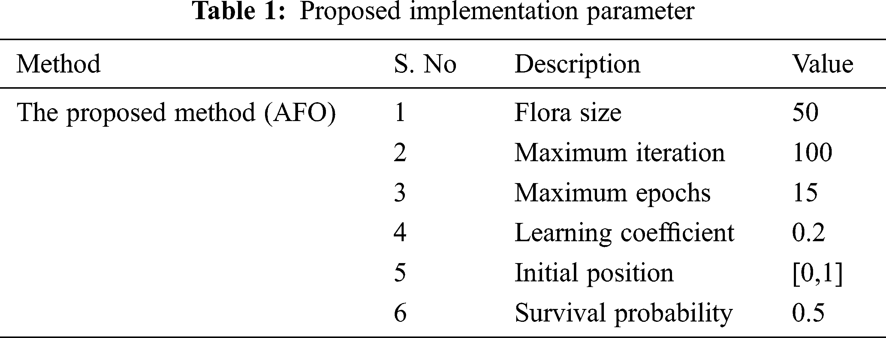
Recommended gene expression data classification is implemented on MATLAB sites. This method uses input database Gene expression Cancer RNA-seq Database and it is available at https://archive.ics.uci.edu/ml/datasets/gene+expression+cancer+RNA-Seq. The measure of information is 801 examples, each characterized by 20,531 highlights. Genes are related to names going from gene_0 to gene_20530. In the proposed method, the dimensional reduction is performed by OLPP, and gene data classification is done by an OLSTM. From the database, gene expression data is classified into five classes: BRCA, KIRC, COAD, LUAD, and PRAD. The proposed implementation parameter is given in Tab. 1.
4.1 Experimental Results Analysis
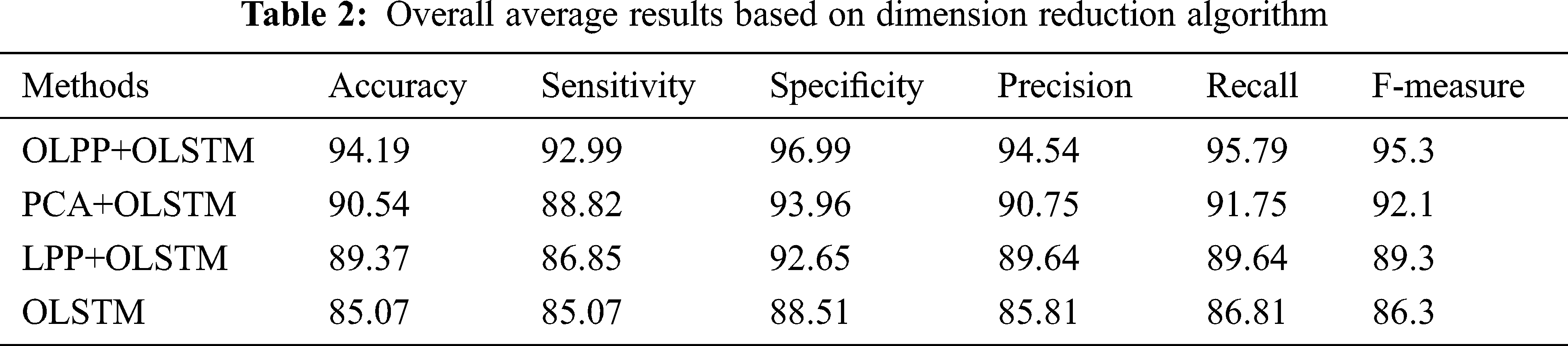
The main objective of proposed approach is to classify a cancer data using dimension reduction and classification algorithm. For dimension reduction, the OLPP algorithm is used here. It reduces the complexity of classification. To assess the performance of proposed dimensionality reduction, PCA and LPP methods are embedded in the OLSTM classifier to carry out the classification diagnosis. The accuracy of a classification and different metrics are shown as follows.
In Fig. 3a, the performance of the suggested method is investigated using accuracy by varying number of iterations. The number of iteration represents in the x-axis and the accuracy value is represented in the y-axis. A good classification system has maximum accuracy. From Fig. 3a, the suggested method achieves a better accuracy of 95.5% which is 92.3% for PCA+OLSTM based classification, 91.4% for LPP+OLSTM, and 86.5% for LSTM based classification. When the number of iteration increases to 50, the proposed method achieves maximum accuracy. And there is no change in the results when the number of iterations exceeded 50. Besides, compared to dimensionality reduction based classification approach getting better compared to without dimensionality reduction approach. From the figure, the accuracy value is increased after dimensional reduction; it is clear that OLPP+OLSTM get higher accuracy compared to the other method. The efficiency of the proposed approach is analyzed based on sensitivity is discussed in Fig. 3b. When analyzing Fig. 3b, the proposed approach attains the maximum sensitivity of 94.5% at iteration 50. Here, the performance is calculated for various dimension reduction approach. Similarly, in Fig. 3c, the efficiency of the suggested model is discussed based on specificity. From the figure, we understand that the recommended technique achieves maximum uniqueness compared to other techniques. The dominant performance of the OLPP is avoiding premature convergence. It also reduces locality and increases globalization under orthogonal control.
The performance of the suggested technique is analyzed based on precision is given in Fig. 3d. High dimensional data are increases the complexity and it will minimize the classification accuracy. Therefore, in this paper, dimensionality reduction is focused. As per Fig. 3d, the suggested technique attained the maximum precision of 96.5% which is 92.3% for PCA+OLSTM based classification, 91.4% for LPP+OLSTM based classification, and 87.5% for OLSTM based classification. As per the analysis, it’s clear that the suggested technique achieved better results compared to the other approaches. This is due to OLPP based dimension reduction process. OLPP overcome the difficulties present in the PCA and LPP. In Fig. 3e, the performance of the suggested technique is analyzed based on Recall. From the figure, when the number of iteration increases to 50, the suggested technique improves the recognition accuracy compared to the existing method. At some point, the number of iteration increases to 50 the suggested recognition accuracy is saturated. Similarly, in Fig. 3f, based on the F-Measure value, the proposed performance is analyzed. Compared to other methods, the suggested method achieves better performance. The test results are analyzed in Tab. 2. The iteration is repeated 100 times, and an average value is taken to compare the classification results. In these results, we have changed the dimension reduction method and the same algorithm OLSTM is used for classification. By changing the dimension reduction method, the results also changed. When analyzing Tab. 2, the proposed approach attained an average accuracy of 94.19%, the sensitivity of 92.09, specificity of 96.99%, the precision of 94.54%, recall of 95.79%, and F-measure of 95.3%. The achieved values are high compared to the other methods. Compared to other methods, the suggested method achieves better performance.

Figure 3: Experimental results, (a) Accuracy, (b) Sensitivity, (c) Specificity, (d) Precision, (e) Recall and (f) F-measure
4.2 Comparative Analysis with Published Work
To demonstrate the effectiveness of the proposed approach, we compare our proposed work with already published research. Here the proposed method considering the existing method is Elbashir et al. [15], Xu et al. [18], and Kong et al. [22]. In [17], the gene expression data classification is done by Lightweight Convolutional Neural Network, and in the existing method [18], Deep Flexible Neural Forest Model is used to detect cancer. A deep feed-forward network is used for gene data classification in the existing method [22].

Figure 4: Comparative analysis of proposed with various research papers
The proposed efficiency is analyzed using accuracy in Fig. 4. Here, we compare our research work with already published works. When analyzing the above Fig. 4, it is clear that the suggested method reaches the maximum accuracy contrasted to the other state of art methods. Here the recommended method attains the gene expression data classification accuracy of 95.5% but the existing method [15] gets the accuracy value is 94.3% and 93.6% of accuracy value is attained by the existing method [18]. The accuracy value of the current method [22] is 93.8% of the minimum value compared to the recommended method. From the results, it is clear that the recommended method achieves better classification accuracy compared to the level of art methods.
5 Conclusions and Future Scope
Here, the method designed an efficient dimensionality reduction with OLSTM for gene expression data classification. Here the input dataset is downloaded from the UCI machine learning repository. At first, the downloaded data is preprocessed. Then dimensionality reduction is done by OLPP. Finally, gene expression data classification is done by OLSTM. Here the weight is optimized using the AAF method. The proposed genetic expression data classification is implemented in MATLAB. Using accuracy, sensitivity, specificity, accuracy, retraction, and F-measure, the proposed performance is analyzed. From the test results, the efficiency of the gene expression data classification with maximum accuracy value is clearly shown. The OLPP+OLSTM method achieves 95.5% classification accuracy. It is clear from the above results that the proposed method demonstrates that in real-time it is possible to classify genetic expression data with better accuracy compared to other methods. Future work of the proposed method is to improving classifier performance by designing an efficient feature selection algorithm.
Acknowledgement: The author with a deep sense of gratitude would thank the supervisor for his guidance and constant support rendered during this research.
Funding Statement: The authors received no specific funding for this study.
Conflicts of Interest: The author declares that they have no conflicts of interest to report regarding the present study.
1. M. Maniruzzaman, M. Jahanur Rahman, B. Ahammed, M. Abedina, H. S. Suri et al., “Statistical characterization and classification of colon microarray gene expression data using multiple machine learning paradigms,” Computer Methods and Programs in Biomedicine, vol. 176, no. 3, pp. 173–193, 2019. [Google Scholar]
2. L. Huijuan, L. Yang, K. Yan, Y. Xue and Z. Gao, “A cost-sensitive rotation forest algorithm for gene expression data classification,” Neurocomputing, vol. 228, no. 5, pp. 270–276, 2017. [Google Scholar]
3. L. Huijuan, J. Chen, K. Yan, Q. Jin, Y. Xue et al., “A hybrid feature selection algorithm for gene expression data classification,” Neurocomputing, vol. 256, no. 1, pp. 56–62, 2017. [Google Scholar]
4. W. Peng and D. Wang, “Classification of a DNA microarray for diagnosing cancer using a complex network based method,” IEEE/ACM Transactions on Computational Biology and Bioinformatics, vol. 16, no. 3, pp. 801–808, 2018. [Google Scholar]
5. B. S. Haddou, N. Hamdi, A. Zeroual and K. Auhmani, “Gene-expression-based cancer classification through feature selection with KNN and SVM classifiers,” 2015 Intelligent Systems and Computer Vision (ISCV), pp. 1–6, 2015. [Google Scholar]
6. L. Qingzhong, A. H. Sung, Z. Chen, J. Liu, L. Chen et al., “Gene selection and classification for cancer microarray data based on machine learning and similarity measures,” BMC Genomics, vol. 12, no. 5, pp. 1–12, 2012. [Google Scholar]
7. L. Jing, W. Cai and X. G. Shao, “Cancer classification based on microarray gene expression data using a principal component accumulation method,” Science China Chemistry, vol. 54, no. 5, pp. 802–811, 2011. [Google Scholar]
8. M. O. Arowolo, M. O. Adebiyi, A. A. Adebiyi and O. J. Okesola, “A hybrid heuristic dimensionality reduction methods for classifying malaria vector gene expression data,” IEEE Access, vol. 8, pp. 182422–182430, 2020. [Google Scholar]
9. S. S. Wei, H. J. Lu, Y. Lu and M. Y. Wang, “An improved weight optimization and Cholesky decomposition based regularized extreme learning machine for gene expression data classification,” Extreme Learning Machines 2013: Algorithms and Applications, pp. 55–66, 2014. [Google Scholar]
10. Y. Yang, P. Yin, Z. Luo, W. Gu, R. Chen et al., “Informative feature clustering and selection for gene expression data,” IEEE Access, vol. 7, pp. 169174–169184, 2019. [Google Scholar]
11. S. S. Kannan and N. Ramaraj, “A novel hybrid feature selection via symmetrical uncertainty ranking based local memetic search algorithm,” Knowledge-Based Systems, vol. 23, no. 6, pp. 580–585, 2010. [Google Scholar]
12. A. Wahid, D. M. Khan, N. Iqbal, S. A. Khan, A. Ali et al., “Feature selection and classification for gene expression data using novel correlation based overlapping score method via Chou’s 5-steps rule,” Chemometrics and Intelligent Laboratory Systems, vol. 199, no. 16, pp. 103958, 2020. [Google Scholar]
13. S. P. Potharaju and M. Sreedevi, “Distributed feature selection (DFS) strategy for microarray gene expression data to improve the classification performance,” Clinical Epidemiology and Global Health, vol. 7, no. 2, pp. 171–176, 2019. [Google Scholar]
14. P. He, B. Fan, X. Xu, J. Ding, Y. Liang et al., “Group K-SVD for the classification of gene expression data,” Computers & Electrical Engineering, vol. 76, no. 1, pp. 143–153, 2019. [Google Scholar]
15. M. K. Elbashir, M. Ezz, M. Mohammed and S. S. Saloum, “Lightweight convolutional neural network for breast cancer classification using RNA-seq gene expression data,” IEEE Access, vol. 7, pp. 185338–185348, 2019. [Google Scholar]
16. T. Khorshed, M. N. Moustafa and A. Rafea, “Deep learning for multi-tissue cancer classification of gene expressions (GeneXNet),” IEEE Access, vol. 8, pp. 90615–90629, 2020. [Google Scholar]
17. H. Lu, H. Gao, M. Ye and X. Wang, “A hybrid ensemble algorithm combining AdaBoost and genetic algorithm for cancer classification with gene expression data,” IEEE/ACM Transactions on Computational Biology and Bioinformatics, pp. 15–19, 2019. [Google Scholar]
18. J. Xu, P. Wu, Y. Chen, Q. Meng, H. Dawood et al., “A novel deep flexible neural forest model for classification of cancer subtypes based on gene expression data,” IEEE Access, vol. 7, pp. 22086–22095, 2019. [Google Scholar]
19. G. Pilar, I. S. Berriel, J. A. Martínez-Rojas and A. M. Diez-Pascual, “Unsupervised feature selection algorithm for multiclass cancer classification of gene expression RNA-Seq data,” Genomics, vol. 112, no. 2, pp. 1916–1925, 2020. [Google Scholar]
20. L. Sun, X. Zhang, Y. Qian, J. Xu and S. Zhang, “Feature selection using neighborhood entropy-based uncertainty measures for gene expression data classification,” Information Sciences, vol. 502, no. 293, pp. 18–41, 2019. [Google Scholar]
21. R. Wang, F. Nie, R. Hong, X. Chang, X. Yang et al., “Fast and orthogonal locality preserving projections for dimensionality reduction”,” IEEE Transactions on Image Processing, vol. 26, no. 10, pp. 5019–5030, 2017. [Google Scholar]
22. Y. Kong and T. Yu, “A graph-embedded deep feedforward network for disease outcome classification and feature selection using gene expression data,” Bioinformatics, vol. 34, no. 21, pp. 3727–3737, 2018. [Google Scholar]
 | This work is licensed under a Creative Commons Attribution 4.0 International License, which permits unrestricted use, distribution, and reproduction in any medium, provided the original work is properly cited. |