DOI:10.32604/iasc.2022.024192
| Intelligent Automation & Soft Computing DOI:10.32604/iasc.2022.024192 | |
| Article |
Tuning Rules for Fractional Order PID Controller Using Data Analytics
Department of EEE, Thiagarajar College of Engineering, Madurai, Tamilnadu, 625015, India
*Corresponding Author: P. R. Varshini. Email: varshinipapers541@gmail.com
Received: 08 October 2021; Accepted: 16 November 2021
Abstract: Flexibility and robust performance have made the FOPID (Fractional Order PID) controllers a better choice than PID (Proportional, Integral, Derivative) controllers. But the number of tuning parameters decreases the usage of FOPID controllers. Using synthetic data in available FOPID tuners leads to abnormal controller performances limiting their applicability. Hence, a new tuning methodology involving real-time data and overcomes the drawbacks of mathematical modeling is the need of the hour. This paper proposes a novel FOPID controller tuning methodology using machine learning algorithms. Feed Forward Back Propagation Neural Network (FFBPNN), Multi Least Squares Support Vector Regression (MLSSVR) chosen to design Machine Learning based Optimal Tuner (MLOT) can handle the interdependency between the controller parameters and multiple outputs for multiple inputs.The proposed tuner finds application in the control of power and energy systems. It can accomplish tracking, disturbance-rejection, and robustness controller performances, thus making FOPID controller design easier and accurate. Comparisons with existing FOPID tuning rules show better controller performances and easy tuning. Thus, this paper addresses a unique, real-time, model-free, easily tunable FOPID tuning methodology satisfying plant requirements.
Keywords: Machine learning; data analytics; support vector regression; controller tuning rule; multi least squares support vector regression; fractional order PID controller
In most of the process control industries, control loops are of Proportional Integral Derivative (PID) type [1]. A Greater number of failures encountered in industrial controllers are due to poor tuning of PID loops. From literature, it is found that PIDs still provide underperformance in most of the process control loops [2,3]. Fractional Order PID (FOPID) controllers introduced by Podlubny [4] in 1994 are more flexible than PID controllers owing to the two additional parameters, the order of integrator ‘
Due to design flexibility, the FOPID controllers find applications especially in systems having nonlinear dynamics [7–10], systems with long-dead time [11], higher-order systems [12], and also unstable systems.
Even though the FOPID controller is found to outperform the conventional PID controllers, design of FOPID controller can be more difficult as it involves five tuning parameters namely, proportional gain constant ‘
Determination of FOPID controller parameters is achieved using many optimization algorithms [13] and artificial intelligence techniques such as fuzzy, neural networks. These techniques require algorithm execution time and initial ground work like determining membership functions, training of algorithms. A single tuning rule without the need of any mathematical calculations and algorithm execution exists; the computation of controller parameters will be much easier.
In last two decades, tuning rules such as Ziegler-Nichols (ZN), Cohen-Coon and Kappa–Tau are the classical empirical tuning rules for FOPID control parameters. FOPID tuning rules based on optimal load disturbance rejection [14], followed by optimal set point tracking are given in [15,16]. The FOPID tuning rules for integral and unstable processes are also available [17] based on statistical polynomial curve fitting. The statistical polynomial curve fitting requires a representative model having accurate initial estimate of the parameter set. These methods involve very small dataset followed by interpolation of data for curve fitting. Also, these methods offer separate equation for each controller parameter which make the controller design tedious.
In addition to the above said drawbacks, these FOPID tuning rules are devised using very little information on system dynamics, also require prior assumptions, approximations and fail to include robustness.Hence, a more accurate, flexible, easily accessible tuning rule, without the need of any mathematical formulations or initial estimation of parameter set is need of the hour.
Hence to overcome the above-said drawbacks, Machine Learning based Optimal Tuner (MLOT) is proposed in this paper. Machine Learning Algorithm (MLA) is advantageous since, it is the strongest predictive modeling for linear as well as nonlinear patterns, with lesser assumptions supplying a single predictive model [18–20].
In this proposed work, the optimal FOPID controller dataset is generated to achieve two-different performance specifications, Set-Point Tracking (SPT) and Load Disturbance Rejection (LDR) for various First Order Plus Dead Time (FOPDT) systems using Covariance Matrix Adaptive Evolutionary Strategy (CMA-ES) [21].
Data analytics is performed on SPT and LDR datasets to remove outliers if any and to identify the most suitable MLA. Thus, identified MLA accomplishes the task of MLOT. Two MLAs, Feed Forward Back Propagation Neural Network (FFBPNN) [22,23] and Multi-output Least-squares Support Vector Regression Machines (MLSSVR) [24,25] have been identified and MLOT-FFBPNN, MLOT-MLSSVR is devised using the two algorithms. To test the proficiency of the chosen MLA, MLOT is also constructed using Multi-Variate Regression (MVR) [26,27]. The proposed system can be applied to systems with long dead time, higher order systems which is the advantage.
The proposed MLOT is justified in terms of performance specifications, statistical variations in controller parameters obtained from MLAs by comparing with the Tuning Rules (TR) given by Padula and Visioli.
The authors claim, the following points as the novelty of this proposed work.
a) A Universal tuner for FOPID controllers using MLA is proposed.
b) Data analysis with R studio® is used to identify appropriate MLAs.
c) Among the two MLAs, MLSSVR is chosen and verified using statistical analysis.
d) Better tracking, disturbance rejection, and robustness performances were achieved.
e) Proposed MLOT is applicable to the FOPDT system and also to any higher-order systems.
The organization of the paper is as follows. Section 2 describes the proposed methodology. Results and discussions are placed in Section 3 and conclusions are given in Section 4.
The flow diagram of the proposed methodology is given in Fig. 1. Initially, CMA-ES algorithm generates dataset with SPT and LDR objectives constrained with Maximum Sensitivity (Ms). Optimal SPT dataset and LDR dataset are obtained as Kpsp, Tisp, Tdsp, λsp, μsp and Kpld, Tild, Tdld, λld, μld respectively.
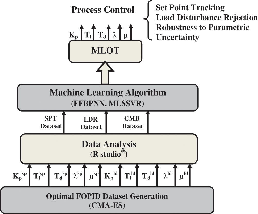
Figure 1: Flow diagram for design of MLOT
The generated dataset is analyzed using R studio for removing outliers and identification of suitable MLAs. MLOT-FFBPNN and MLOT-MLSSVR are formulated with the dataset from the data analysis block which is applicable to any process control system.
2.1 Optimal FOPID Dataset Generation
Optimal FOPID dataset is generated by optimizing the FOPID controller design for a range of FOPDT systems FOPDT1, FOPDT2, …FOPDTn. The CMA-ES algorithm is used for optimization with seven different maximum sensitivity values, Ms = [1.4, 1.5, 1.6, 1.7, 1.8, 1.9, 2.0] under two design objectives, SPT and LDR. The FOPDT system is in the form of Gp as given in Eq. (1) with process gain ‘K’, time constant ‘T’, dead time ‘L’ and also, normalized dead time, τ = L/ (L + T). The τ is associated with the dynamic behavior of a FOPDT system.
Hence, the ‘n’ number of different FOPDT systems (FOPDT1, FOPDT2, … FOPDTn) are produced by varying τ as τ1,τ2,…τn between the range [0.3, 0.8]. The structure of FOPID controller used is given in Eq. (2) and Oustaloup approximation in Eq. (3)
The FOPID controller parameters are obtained for ‘n’ different FOPDT systems by minimizing the Integral Absolute Error (IAE). CMA-ES [25,26] optimization algorithm is used to minimize IAE in Eq. (4) for the two performance objectives namely, SPT to obtain minimum IAEsp and LDR to obtain minimum IAEld as in Eq. (5).
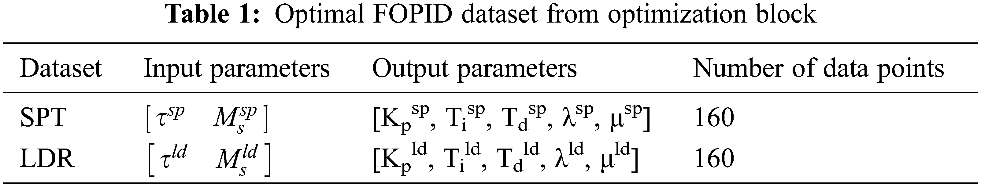
The dataset generated from the optimization block will be of the form as given in Tab. 1. Both SPT and LDR objectives are optimized for 160 numbers of different FOPDT systems and hence 160 numbers of SPT and LDR data points are obtained respectively and this is provided in the last column of Tab. 1. The variables [τ, Ms] are chosen as input parameters while [Kp, Ti, Td, λ, μ] are chosen as the output parameters.
2.2 Data Analysis of Generated Optimal FOPID Dataset
To design MLOT, an MLA that can handle many inputs with many output parameters is required. Before using such MLA, the inter-variable correlation between the output parameters must be determined to obtain an efficient machine learning model. Also, the dataset generated from the optimization block may contain few data points that may differ from other observations termed outliers. Outliers may be due to measurement error which must be discarded to avoid misleading of modeling. Data analysis using R studio® is carried out in this work to check and discard any outliers, and also to analyze the relationship between the output parameters of the generated dataset.
For a multiple input multiple output model, some data may be suitable in a single dimension but they may become an outlier in a multi-dimension. The Cook’s distance identifies the presence of outliers. These outliers are then removed from the dataset by identifying the data points having standard deviations greater than the mean value.
2.2.2 Cross-Correlation among Output Parameters
The SPT and LDR dataset contains four output variables. The cross-correlation matrix of these four output variables for the SPT dataset after removing outliers is obtained. Positive/Negative large cross-correlation values denote high linear interrelationship among the variables. A Smaller cross-correlation value does not mean that the corresponding parameter is an independent one. For such cases, the cross-correlation plots have to be examined for non-linear relations. Hence, in this work, both the cross-correlation matrix values and the cross-correlation plots have been analyzed for determining the interrelationship among the output parameters before modeling with MLAs.
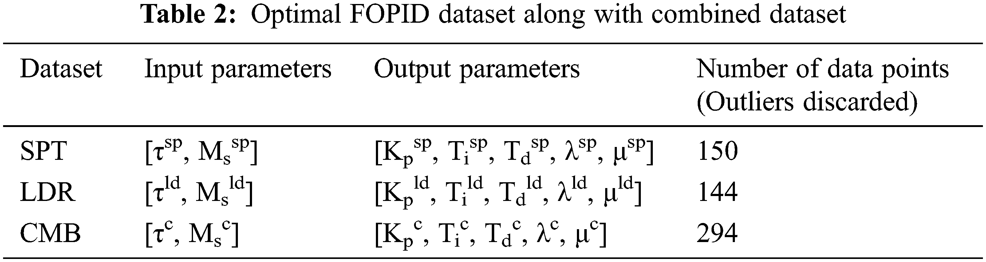
The SPT and LDR dataset are combined together to obtain the third dataset, the CMB dataset from the generated data points as given in Tab. 2. In the CMB dataset, τc = [τsp, τld] while Msc = [Mssp, Msld]. Also, Kpc = [Kpsp, Kpld], Tic = [Tisp, Tild], Tdc = [Tdsp, Tdld], λc = [λsp, λld], μc = [μsp, μld].
Data analysis results confirm a high cross-correlation among output parameters. Two MLAs, FFBPNN and MLSSVR have been identified to support the highly correlated dataset. FFBPNN and MLSSVR are employed to design the proposed MLOT using the three datasets obtained from the data analysis block.
In FFBPNN, the Levenberg-Marquardt function with Mean Square Error (MSE) minimization is considered. In MLSSVR multi-tasking is achieved by using weight vector, wi = w0 + vi, where, wi ∈ R. w0 is the regular weight vector that determines the output while
The three MLAs are compared based on their statistical parameters such as Correlation Coefficient (CC), Mean Square Error (MSE), Root Mean Square Error (RMSE), and Mean Absolute Error (MAE). The results of MLOTs are also compared with the existing FOPID tuning rule. The MATLAB® program to evaluate FOPID controller parameters using the proposed MLOT is available with the authors. This MATLAB® program can be used to determine FOPID controller parameters for any FOPID and higher-order systems.
An Intel® Core™ i7-3632 QM CPU with 2.2 GHz speed and 8 GB RAM computer with 8 logical processors is used to develop the proposed MLOT in this paper. The optimization is carried out with the help of the MATLAB® toolbox while the data analysis is performed using R studio®.
3.1 Optimization/Dataset Generation
The FOPDT system parameters K and T are set to 1. Different FOPDT systems are considered for dataset generation with different τ ϵ [0.3, 0.8].
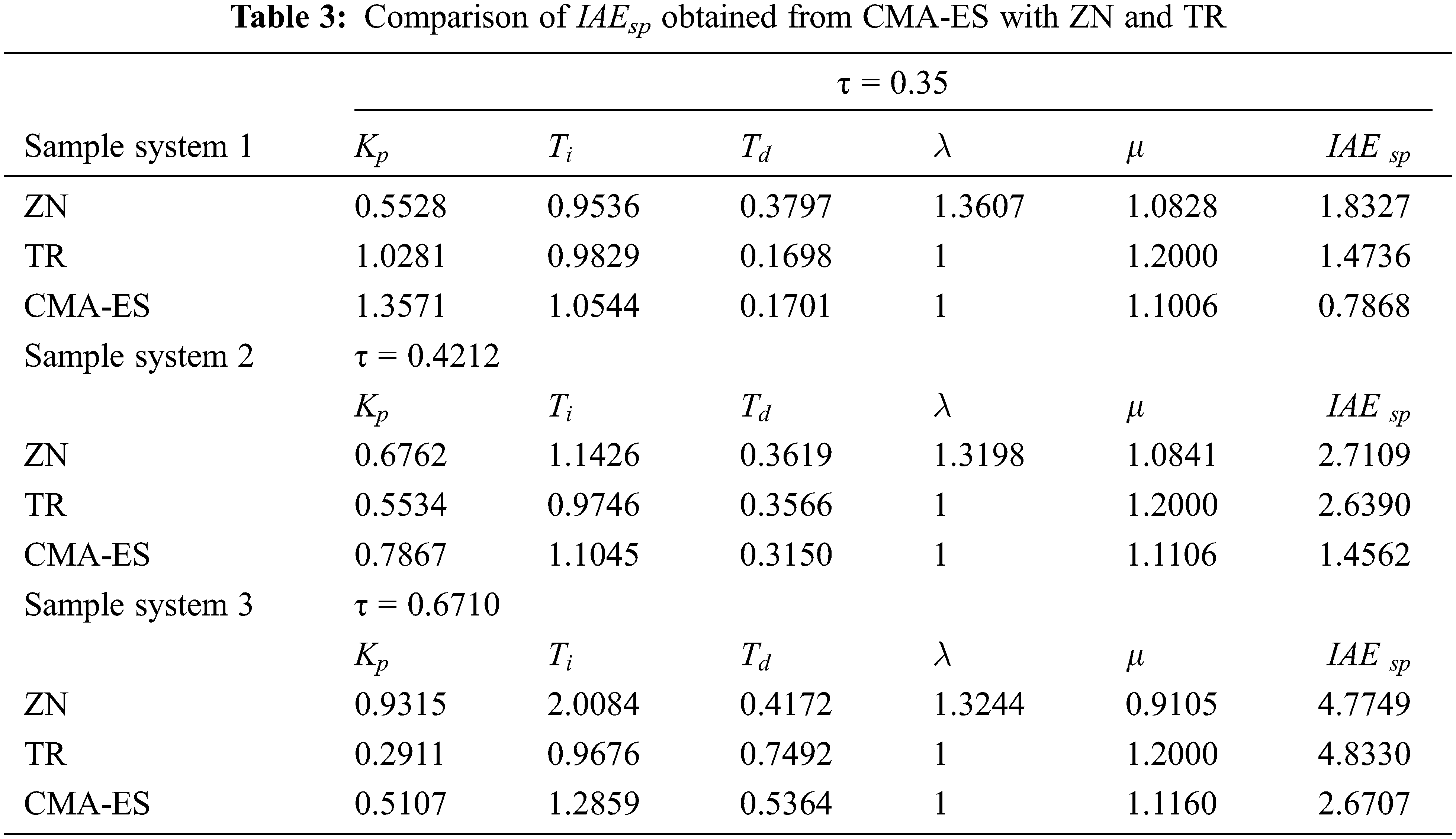
The optimum values of IAEsp obtained from CMA-ES for various FOPDT sample systems are compared with the results obtained from ZN rules and TR given by Padula and Visioliin Tab. 3. The comparison is given for three example systems. It is observed from Tab. 3, IAEsp is minimum for the CMA-ES method, in all three FOPDT sample systems.
The graphs in Fig. 2 confirm that the optimal controller parameters obtained using the CMA-ES algorithm are found to vary smoothly for τ in both the design objectives.
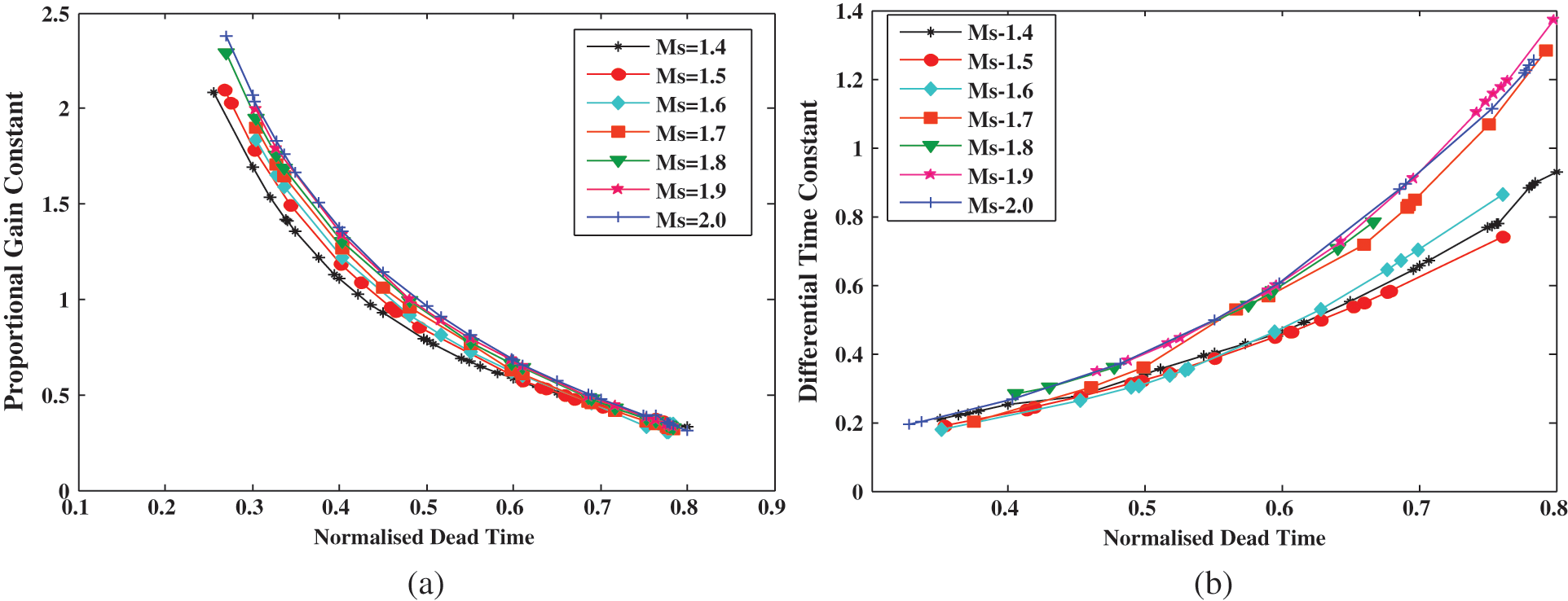
Figure 2: Parameter variation for various FOPDTs. (a) KpspVs τ for SPT (b) TdldVs τ for LDR
The input and output variables of the SPT and LDR dataset are given in Table I for developing the MLAs. Based on Cook’s distance, outliers present in the Kp parameter of the SPT dataset are identified and denoted by the red colour ‘+’ (plus) symbol as shown in Fig. 3a data points after removing outliers are given in Fig. 3b. Similarly, outliers are removed in LDR dataset also.
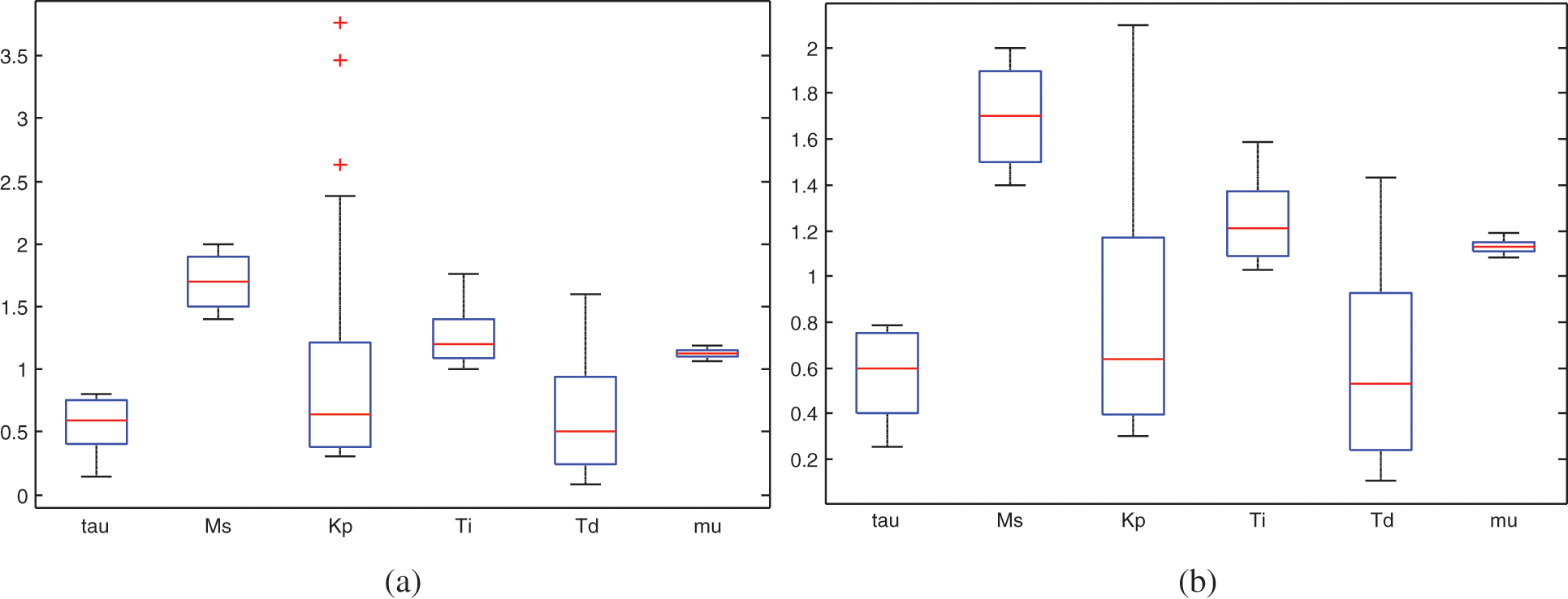
Figure 3: Box plot for SPT dataset. (a) With outliers (b) without outliers
The cross-correlation matrix of the four output variables for the SPT dataset after removing outliers is given in Tab. 4. The diagonal plots in Fig. 4 represent the histogram of the data distribution for each output variable. The lower diagonal plots represent the variation between the output variables. The upper diagonal represents their cross-correlation values similar to that tabulated in Tab. 4. The font size is larger for large cross-correlation values while font size is smaller for lower values of cross-correlation in Fig. 4. The red-colored ‘***’ represents very large cross-correlation values among all.
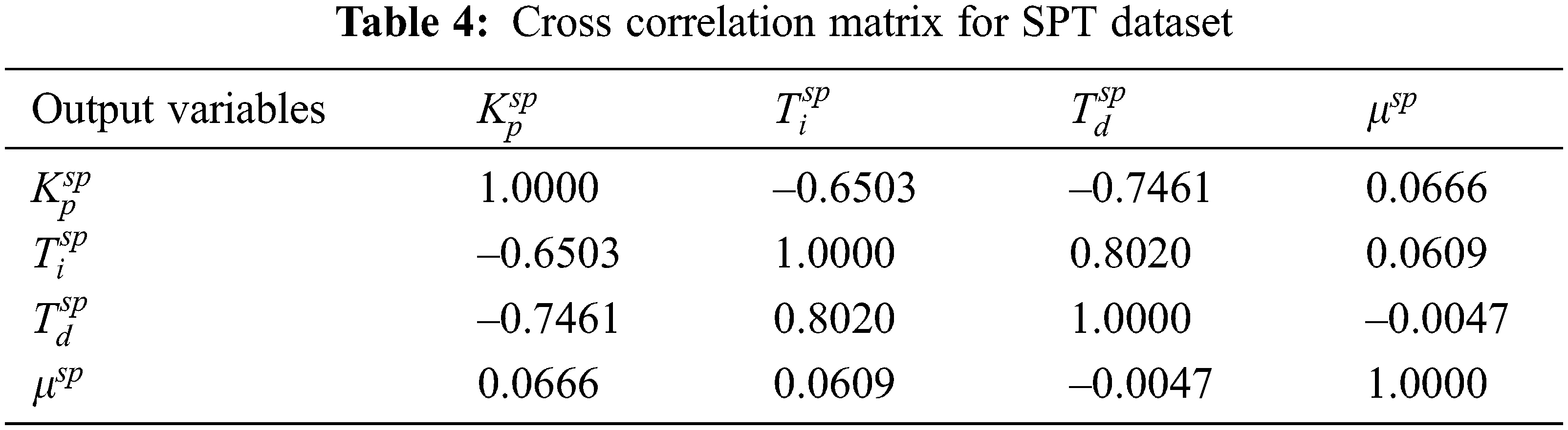
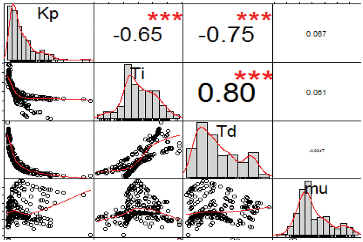
Figure 4: SPT dataset-cross correlation matrix
3.3 Development of MLOT Models
The three MLAs, MLOT-FFBPNN, MLOT-MLSSVR, MLOT-MVR algorithms for SPT, LDR, and CMB datasets are used to develop totally nine MLOT models. The MLOT models are tested using randomly generated data points named testing data points that are not involved in the training and validation phase. Figs. 5a and 5b shows the variation of Tdld, μld with respect to τld for MLOT-LDR.
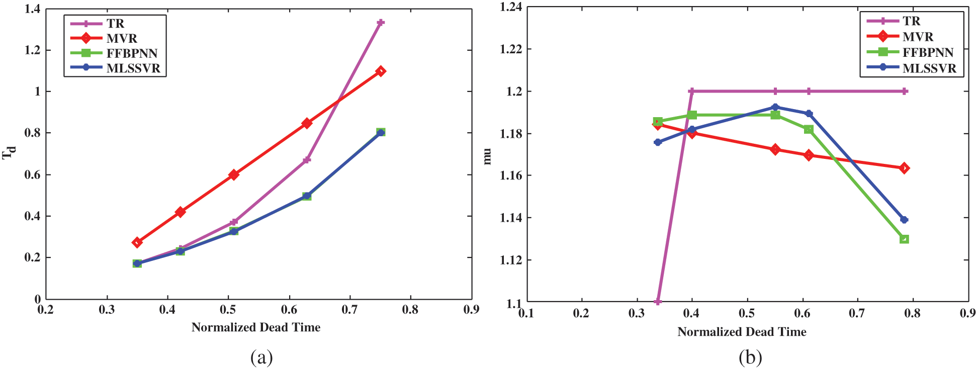
Figure 5: Validation results of three MLOT models compared with results from TR. (a) TdldspVsτld from MLOT-LDR (b) μldVsτld from MLOT-LDR
Also, it can be observed that the results of testing data points in Fig. 6 follow the graphs of parameter variations similar to the validation data points in Fig. 5. Also, the results from TR show that controller parameters from FFBPNN and MLSSVR are closer to the optimum controller parameters than the results from TR.
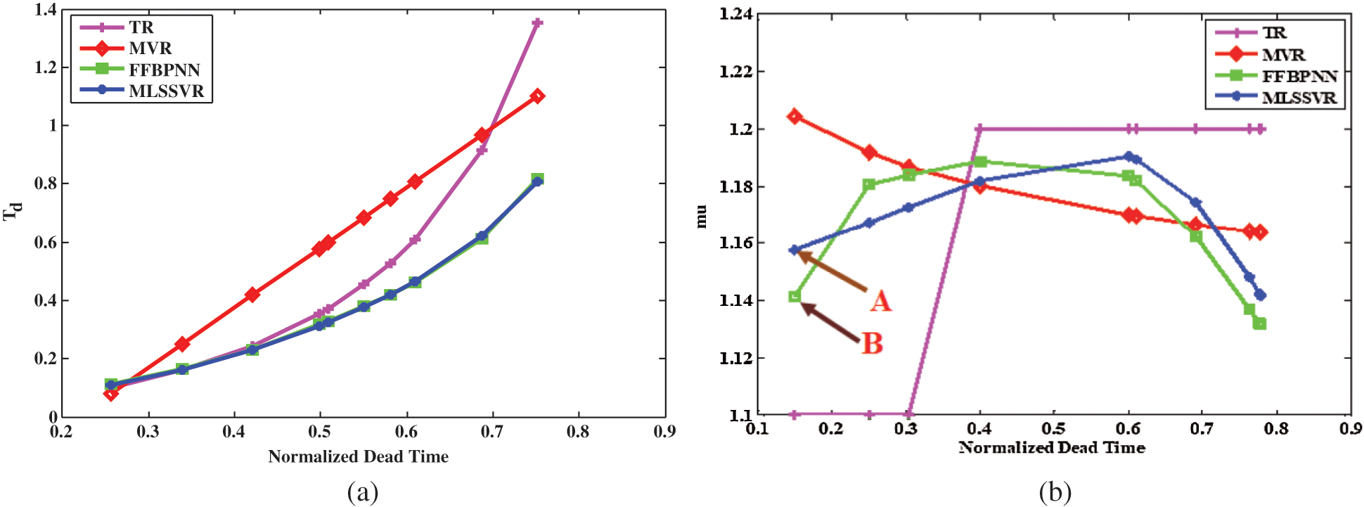
Figure 6: Testing results of three MLOT models compared with results from TR. (a) TdldVsτld from MLOT-LDR (b) μldVsτld from MLOT-LDR
In graph μldVsτldof Fig. 6b for Ms = 2.0, the point A indicates the value of μld from MLSSVR (blue color) and point B from FFBPNN (green color) for the same value of τld = 0.15. But, point A and point B clearly indicate that FFBPNN (green color) does not follow the pattern as given in Fig. 5b when compared to MLSSVR (blue color). This indicates that the MLSSVR algorithm produces better results than FFBPNN.
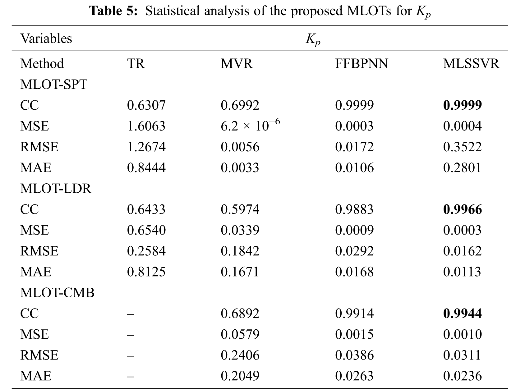
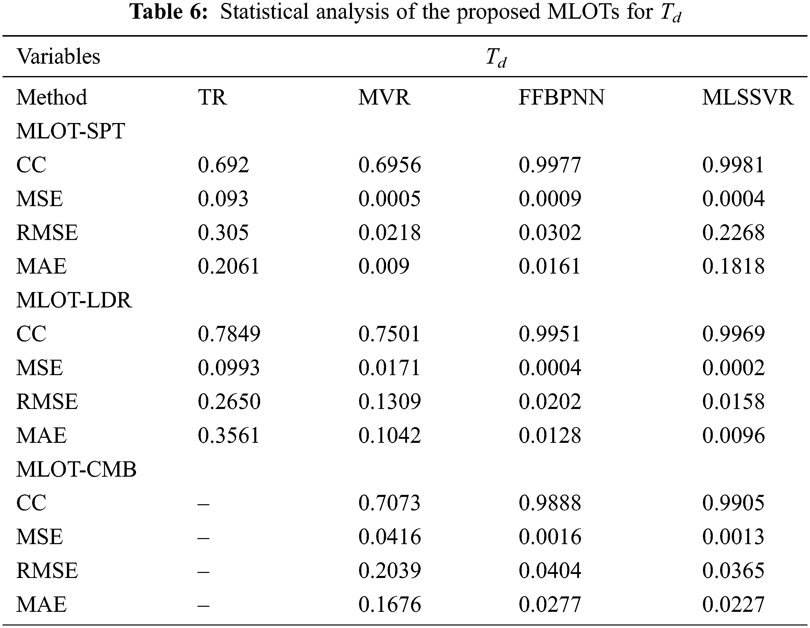
The statistical performances of proposed MLOTs are better than TR and MVR as given in Tab. 5 for Kp and Tab. 6 for Td.
The statistical results of controller parameters are given as spider graphs in Figs. 7 and 8. For a better machine learning model, the CC values must be very large and the MSE, RMSE, MAE values must be the least. The CC values for all the output parameters in MLSSVR are larger compared to all other methods. This is shown by the outermost web denoted by red colour in Fig. 7a. Also, the MSE values of MLSSVR results are the least and it is given by the innermost web given in Fig. 7b denoted in red colour.
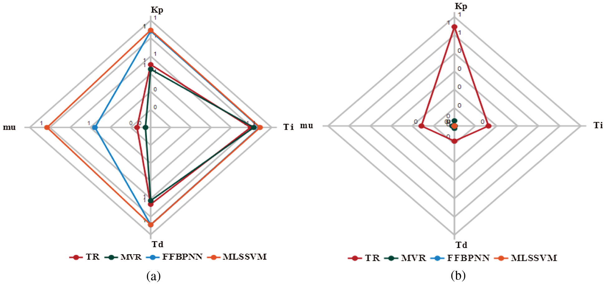
Figure 7: MLOT-LDR dataset. (a) CC (b) MSE
The CC values for the CMB dataset are compared among MLOT-MLSSVR, MLOT-FFBPNN, MLOT-MVR models in Fig. 8a. The MLOT-MLSSVR takes the outermost spider web (red colour) denoting larger correlations among the generated CMA-ES controller parameters and the controller parameters from validation data. Similarly, the results from MLOT-MLSSVR have the least MSE while using the CMB dataset. This is denoted by the innermost spider web given in red colour as shown in Fig. 8b.
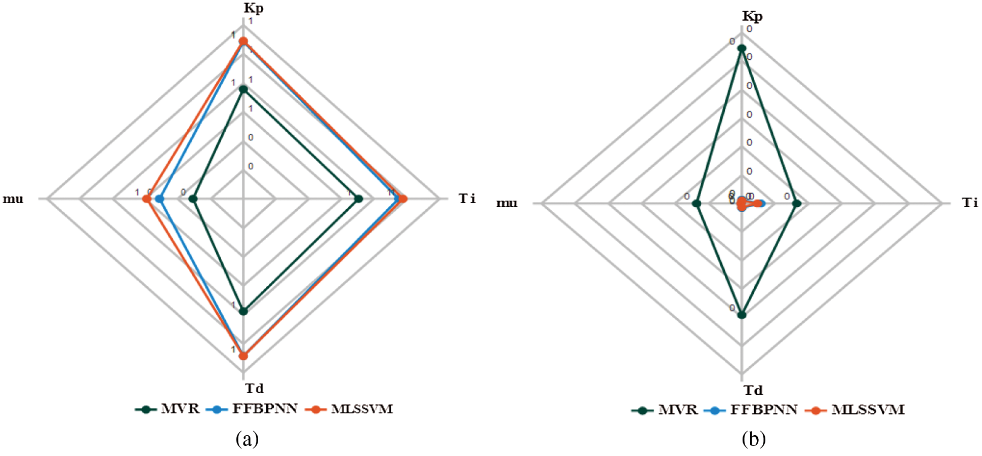
Figure 8: MLOT-CMB dataset. (a) CC (b) MSE
This paper proposes a novel FOPID controller tuning methodology using machine learning algorithms. Feed Forward Back Propagation Neural Network (FFBPNN), Multi Least Squares Support Vector Regression (MLSSVR) chosen to design Machine Learning based Optimal Tuner (MLOT) can handle the interdependency between the controller parameters and multiple outputs for multiple inputs. The statistical analysis values reveal that, the CC values of MLSSVR is 0.999, 0.9966, 0.9944 for MLOT-SPT, MLOT-LDR, MLOT-CMB for Kp. The MLOT-MLSSVR using the CMB dataset perfectly captures variations among controller parameters. The graphical analysis of parameter variations and statistical analysis confirms the better results for the proposed MLOT over the FOPID Tuning Rule (TR) given by Padula and Visioli. The proposed MLOT is also applicable for dead time-dominated systems and lag-dominated systems. Pre-processing with large amount of dataset consumes computational time which can be overcome using cloud computing and big data analysis in future.
Acknowledgement: The author with a deep sense of gratitude would thank the supervisor for his guidance and constant support rendered during this research.
Funding Statement: The authors received no specific funding for this study.
Conflicts of Interest: The authors declare that they have no conflicts of interest to report regarding the present study.
1. K. J. Åström and T. Hägglund, PID controllers: Theory, design, and tuning. In: Automatic Tuning of PID Controllers, 2nd ed., Research Triangle Park, NC: Instrument society of America, pp. 1–354, 1995. [Google Scholar]
2. A. O’Dwyer, Handbook of PI and PID controller tuning rules, 3rd ed., USA: Imperial college press, p. 624, 2009. [Google Scholar]
3. P. Shah and S. Agashe, “Review of fractional PID controller,” Mechatronics, vol. 38, no. 7, pp. 29–41, 2016. [Google Scholar]
4. I. Podlubny, “Fractional-order systems and fractional-order controllers,” Institute of Experimental Physics, Slovak Academy of Sciences, Kosice, vol. 12, no. 3, pp. 1–18, 1994. [Google Scholar]
5. C. A. Monje, Y. Chen, B. M. Vinagre, D. Xue and V. Feliu-Batlle, Fractional-order systems and controls: Fundamentals and applications. In: Advances in Industrial Control. London: Springer Science & Business Media, Springer, p. 415, 2010. [Google Scholar]
6. S. Das, S. Saha, S. Das and A. Gupta, “On the selection of tuning methodology of FOPID controllers for the control of higher order processes,” ISA Transactions, vol. 50, no. 3, pp. 376–388, 2011. [Google Scholar]
7. R. V. Yohanandhan and L. Srinivasan, “Decentralised wide-area fractional order damping controller for a large-scale power system,” IET Generation, Transmission & Distribution, vol. 10, no. 5, pp. 1164–1178, 2016. [Google Scholar]
8. S. Debbarma and A. Dutta, “Utilizing electric vehicles for LFC in restructured power systems using fractional order controller,” IEEE Transactions on Smart Grid, vol. 8, no. 6, pp. 2554–2564, 2016. [Google Scholar]
9. I. M. Mehedi, U. M. Al-Saggaf, R. Mansouri and M. Bettayeb, “Two degrees of freedom fractional controller design: Application to the ball and beam system,” Measurement, vol. 135, no. 3, pp. 13–22, 2019. [Google Scholar]
10. H. P. Ren, J. T. Fan and O. Kaynak, “Optimal design of a fractional-order proportional-integer-differential controller for a pneumatic position servo system,” IEEE Transactions on Industrial Electronics, vol. 66, no. 8, pp. 6220–6229, 2018. [Google Scholar]
11. M. H. Khooban, M. ShaSadeghi, T. Niknam and F. Blaabjerg, “Analysis, control and design of speed control of electric vehicles delayed model: Multi-objective fuzzy fractional-order PI λD μ PIλDμ controller,” IET Science, Measurement & Technology, vol. 11, no. 3, pp. 249–261, 2017. [Google Scholar]
12. A. Asgharnia, A. Jamali, R. Shahnazi and A. Maheri, “Load mitigation of a class of 5-MW wind turbine with RBF neural network based fractional-order PID controller,” ISA Transactions, vol. 96, no. 8, pp. 272–286, 2020. [Google Scholar]
13. D. S. Acharya and S. K. Mishra, “A multi-agent based symbiotic organisms search algorithm for tuning fractional order PID controller,” Measurement, vol. 155, no. 9–10, p. 107559, 2020. [Google Scholar]
14. Y. Chen, T. Bhaskaran and D. Xue, “Practical tuning rule development for fractional order proportional and integral controllers,” Journal of Computational and Nonlinear Dynamics, vol. 3, no. 2, p. 021403, 2008. [Google Scholar]
15. F. Padula and A. Visioli, “Optimal tuning rules for proportional-integral-derivative and fractional-order proportional-integral-derivative controllers for integral and unstable processes,” IET Control Theory & Applications, vol. 6, no. 6, pp. 776–786, 2012. [Google Scholar]
16. F. Padula and A. Visioli, “Set-point weight tuning rules for fractional-order PID controllers,” Asian Journal of Control, vol. 15, no. 3, pp. 678–690, 2013. [Google Scholar]
17. F. Padula and A. Visioli, “Tuning rules for optimal PID and fractional-order PID controllers,” Journal of Process Control, vol. 21, no. 1, pp. 69–81, 2011. [Google Scholar]
18. I. H. Witten, E. Frank, M. A. Hall, C. J. Pal and M. Data, “Practical machine learning tools and techniques”. Data Mining, vol. 2, pp. 4, 2005. [Google Scholar]
19. B. J. Perry, Y. Guo, R. Atadero and J. W. van de Lindt, “Streamlined bridge inspection system utilizing unmanned aerial vehicles (UAVs) and machine learning,” Measurement, vol. 164, p. 108048, 2020. [Google Scholar]
20. R. Abdelaziz, M. Elhoseny, A. S. Salama and A. M. Riad, “A machine learning model for improving healthcare services on cloud computing environment,” Measurement, vol. 119, no. 3, p. 117–128, 2018. [Google Scholar]
21. N. Hansen, The CMA evolution strategy: A comparing review. In: Towards a New Evolutionary Computation. Vol. 192. Berlin, Heidelberg: Springer, pp. 75–102, 2006. [Google Scholar]
22. M. H. Beale, M. T. Hagan and H. B. Demuth, Neural network toolbox user’s guide. In: Math Works Inc. Natick, MA: Ver. 4, 2011. [Google Scholar]
23. D. Svozil, V. Kvasnicka and J. Pospichal, “Introduction to multi-layer feed-forward neural networks,” Chemometrics and Intelligent Laboratory Systems, vol. 39, no. 1, pp. 43–62, 1997. [Google Scholar]
24. S. Xu, X. An, X. Qiao, L. Zhu and L. Li, “Multi-output least-squares support vector regression machines,” Pattern Recognition Letters, vol. 34, no. 9, pp. 1078–1084, 2013. [Google Scholar]
25. X. Zhu and Z. Gao, “An efficient gradient-based model selection algorithm for multi-output least-squares support vector regression machines,” Pattern Recognition Letters, vol. 111, no. 5, pp. 16–22, 2018. [Google Scholar]
26. C. Chatfield and A. J. Collins, Introduction to Multivariate Analysis. In: Mathematics & Statistics, 1st ed., Boca Raton: Routledge, pp. 1–248, 1980. [Google Scholar]
27. V. Valério, D. Duarte and J. S. Da Costa, “Tuning of fractional PID controllers with Ziegler-Nichols-type rules,” Signal Processing, vol. 86, no. 10, pp. 2771–2784, 2006. [Google Scholar]
 | This work is licensed under a Creative Commons Attribution 4.0 International License, which permits unrestricted use, distribution, and reproduction in any medium, provided the original work is properly cited. |