Intelligent Automation & Soft Computing DOI:10.32604/iasc.2022.024234
Article

Spectral Vacancy Prediction Using Time Series Forecasting for Cognitive Radio Applications

Vineetha Mathai* and P. Indumathi

Department of Electronics Engineering, Madras Institute of Technology, Anna University, Chennai, 600044, India
*Corresponding Author: Vineetha Mathai. Email: vineethamathai@gmail.com
Received: 10 October 2021; Accepted: 21 December 2021

Abstract: An identification of unfilled primary user spectrum using a novel method is presented in this paper. Cooperation among users with the utilization of machine learning methods is analyzed. Learning methods are applied to construct the classifier, which selects the suitable fusion algorithm for the considered environment so that the out of band sensing is performed efficiently. Sensing performance is looked into with the existence of fading and it is observed that sensing performance degrades with fading which coincides with earlier findings. From the simulation, it can be inferred that Weibull fading outperforms all the other fading models considered. To accomplish missed detection probability of 1% in the Rayleigh channel, the false alarm probability obtained is almost 0.8 however to obtain the same missed detection probability in the Weibull channel, false alarm probability is less than 0.1 which is very favorable for both indoor and outdoor scenarios. Numerical analyses are carried out here to predict Primary User (PU) channel condition using Hidden Markov Model with the help of Time series forecasting learning method. It is evident that the prediction performance has reached 100% as the result of using the Weibull Fading Model for a period of 200 ms when compared to the Rayleigh model which is achieving only 84.5% accuracy in prediction.

Keywords: Co-operative spectrum sensing; machine learning; decision fusion; weibull fading; time series; HMM

1  Introduction

When the spectrum is underutilized, Cognitive Radio (CR) is applied to exploit spectrum holes. This permits the secondary users (SU) along with Primary Users (PU) to approach an unoccupied space in an adaptable style [1]. To observe radio frequencies incessantly Spectrum Sensing (SS) [2] is used. The detection method is used to recognize the availability of PU by computing the received signal energy by applying an Energy Detector (ED) [3]. To mitigate the hidden terminal problem and shadowing effects, the Cooperative Spectrum Sensing (CSS) [4] technique is introduced where numerous CRs in the system feel the presence of PU as shown in Fig. 1. In CSS, for creating decisions CR users interchange sensing outcomes to the Fusion Center (FC). The CR users interchange information to check whether the acquired energy is more than the threshold. Estimated energy is transferred to the fusion center to create an improved decision by using several hard [5–8] and soft-decision algorithms. The FC gives a global result by merging the individual decisions from each CRs.

Figure 1: Proposed schematic for cooperative sensing

Using extended generalized-K distribution fading channels are modeled for spectrum sensing using ED in [9]. The CSS model with an Improved ED (IED) scheme is reviewed in [10] uses several antennas at each CR. The CSS model with an antenna at every CR over the Rician channel is explored in [11]. System parameter performance with an IED scheme is examined over channel models is done in [12]. The analogous study in [13–16] using Nakagami-m and Weibull fading channel with ED method is done since it does not require prior information about the channel. A classifier [16] with energy statistics of PU along with decisions about the existence of PU is used for training. Based on learning methods classifiers can be classified as supervised and unsupervised methods. The unsupervised machine learning technique we used is the K-means algorithm to study and find out the primary user’s data and patterns. The supervised machine learning techniques we used here is SVM to train the model with the data labeled in the previous step. To forecast the decisions on undetected PU channel conditions, the trained classifier is used. Evaluating the PU channel state [17–21] in CR is a tedious job since it is time varying. A lot of works approach on earlier discussed problem [22–24] using Fast Fourier transform (FFT). It is having high complexity because of large computations. Here we introduce the time series forecasting method for identifying the occupancy of the PU channel state. A time series [25] is used to study the PU channel state (i.e., “idle” or “occupied”). Then Hidden Markov Model (HMM) model is used to capture PU channel status [26,27].

Here, we suggest a novel model based on Machine Learning (ML) techniques to detect the unused spectrum of primary users effectively. We consider “energy vector”, as a feature vector in which the energy level is calculated at each CR. Then, the classifier classifies the vector into either the “channel available class” or the “channel unavailable class”. We investigated impact of small-scale fading such as multi-path fading, delay spread and Doppler spread are considered over different fading channels. We examined the performance of an unsupervised machine learning algorithm as well as a supervised machine learning algorithm to construct the classifier for decision making. A qualitative performance evaluation of various fusion methods with learning is presented. To acquire the advantage of multi-path propagation, energy detection with receiver diversity is considered and analysis in terms of missed detection and false alarm probabilities over various fading channels is done. Using HMM, primary user channel state prediction is carried out. To our knowledge, no literature considers both sensing and reporting channels as fading models and includes ML methods for classification and further to foresee next state of PU channel using the time series forecasting method.

The rest of the paper is organized as below. In Section 2 we introduce the signal model and the proposed cooperative spectrum sensing scheme. Different classification and fusion methods are presented. Simulation results and discussions are given in Section 3 discusses the experimental outcomes. Finally, conclusion is given at Section 4.

2  System Model

CR network with a single PU and seven SUs is considered. Here the PU alternates between the idle and busy states. The SU knows the presence of the PU by sensing signals using an ED technique. The signal energy is used to predict the presence of PU. We consider a cooperative CR network with K nodes considering N test points for the ED and M frames for training the ML classifier, as illustrated in Fig. 2.

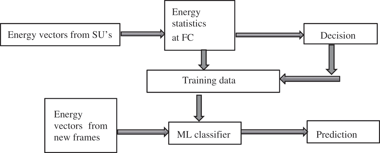
Figure 2: Proposed ML classifier model

The ith frame of the received signal at the jth cooperative node, Yij(n) is given by

Yij(n)= {wij(n)  H0γijSij(n)+wij(n)H1 (1)

where Sij (n) is the primary user’s signal, which is a Gaussian i.i.d random process with zero mean, wij (n) is the noise. The nodes are sensing frame and obtain the statistics. For ith frame at the fusion center, the energy samples Yij, is expressed as γi=1N∑n=1N⁡|Yij(n)|2 , i lies between 1 and M, where γi is a random variable that has a pdf with chi-square distribution. γij is the signal-to-noise ratio of the ith frame observed at the jth cooperative node. σj2 is standard deviation of noise samples wij (n). For all frames, noise variance and SNR remains unchanged during the training process is our assumption. For each frame in the training set a threshold, λj is selected then the probability of the false alarm, Pfa is obtained as

Pfa(λj)= Q((λjσj2−1)) (2)

and probability of detection Pd is

pd(λj)= Q((λjσj2(1+γj)−1)N2) (3)

where Q (.) is the complementary distribution function.

2.1 Fusion Center Threshold Calculation for Various Data Fusion Rules

In order to achieve optimal threshold, λ fusion rules are considered here. K nodes work together for computing the threshold to build the overall sensing decision. The following hard fusion rules are used in the decision center of the secondary users.

2.1.1 AND Fusion Rule

All nodes detect the signal and inform it to FC then, this rule decides that the signal is present so the threshold [2] is

λAND=(2NQ−1(pf1k)+1)σu2 (4)

the detection probability Pd AND [7] can be expressed as

PdAND=(Q((λANDσu2+(1+γu)−1)N2))K (5)

2.1.2 OR Fusion Rule

If one among many users detect the signal, then this rule determines that signal is present so the threshold [2] is

λOR=(2NQ−1(1−(1−pf)1k)+1)σu2 (6)

the detection probability PdOR [7] can be

PdOR=(1−(1−Q(λORσu2+(1+γu)−1)N2))K (7)

The soft fusion rules we considered here include maximum ratio combining (MRC) and square law selection (SLS).

2.1.3 Maximum Ratio Combining (MRC)

All CRs transmit their corresponding vectors to the FC. It gathers the data, combines them, creates a global decision by comparing the value with the detection threshold. The fusion center adds them after receiving these energy statistics γsi=∑j=1K⁡wjγij for i varies from 1 to M where γij is ith frame energy test statistics. To maximize the detection probability, the optimum weight vector, wj has to be obtained. The weighting coefficient vector wj can be achieved as wj = sign(gT w0) w0 where gT=[σ12γ1,σ22γ2,…,σK2γK] with instantaneous SNRs and noise variances. Then fusion threshold is

λMRC=(∑j=1K⁡wjσj2)Q−1[Pf]+∑j=1K⁡wjσj2 (8)

the detection probability PdMRC is given by

PdMRC= Q((λMRC∑j=1K⁡(1+γj)wjσj2−1)N2) (9)

2.1.4 Square Law Selection Rule (SLS)

FC chooses the user with maximum SNR, γSLS [7] with noise variance, σu2 . Then the threshold is given by

λSLS=(2NQ−1(1−(1−pf)1k)+1)σu2 (10)

the detection probability PdSLS is given by

PdSLS=(1−(1−Q(λSLSσu2+(1+γSLS)−1)N2))K (11)

2.2 ML Based Classification Methods

From the energy vectors obtained is compared with the threshold to obtain the decision, di which is linked with ith frame is mentioned as

di= {1γc≥λ−1γc≤λ (12)

where γc∈{γi,γsi} and λε{λAND, λOR,λMRC, λSLS}. Here “−1 “ expresses the PU at rest, and “1” expresses busy PU communication on channel as mentioned in Eq. (12). For classification problem ML based classifier can be used to perceive the decision linked with a new frame. Initially, K-means is applied to find primary users’ transmission patterns and statistics. Then, to differentiate between two states i.e., active or inactive state of the primary user signal, the Support Vector Machine (SVM) method is adopted. In the first step, unsupervised machine learning techniques are used to analyze the primary user’s data and patterns. Further, supervised machine learning techniques are used to train the model with the data labeled in the previous step.

2.2.1 K-Means Clustering

This method divides a group of the training energy vectors into clusters. The set of those vectors that fit in to cluster k is denoted by Ck. It’s centroid is αk. It aims to select K clusters, C1, . . . , CK, which minimize

argminC1,...,Ck⁡∑k=1K⁡∑y∈Ck∥yl−αk∥2 (13)

The steps involved in finding clusters that satisfy Eq. (13) are

1)   The centroids for clusters are initialized first and its value in cluster 1 is fixed as α1 = μY|S . From the cluster set, one cluster is selected that PU is idle (i.e., S = 0) so it belongs to channel available, whereas further clusters belong to unavailable class.

2)   From the energy vectors assigned earlier, centroids are calculated and are updated by obtaining the average of all vectors except for cluster 1.

3)   The iterations are recalculated till it converges. By K-means algorithm centroid for cluster k is obtained as αk∗ =  |Ck|−1∑yl∈Ck⁡yl, ∀k = 2,…,K. After the training it receives the test energy vector, y∗ for further classification. Then classifier decides whether it is a part of cluster 1 or not, by computing distance from the test vector to the centroids.

∥y∗−α1∗∥mink=1,…,K∥y∗−αk∗∥≥β (14)

where parameter β is the threshold to limit the compromise between the misdetection and the false alarm probabilities.

2.2.2 Support Vector Machine

These are supervised learning models and is used to produce the best decision boundary which can separate space into classes. This boundary is called hyperplane. The way of choosing vectors that aid in creating the boundary. These extreme vectors are called support vectors. The dataset of n points is given in the form of (x1, y1),…,(xn, yn) and the final choice is either 1 or −1 that denotes the class to which xi belongs [16] based on the hyperplane equation as

w.x−b = 0  (15)

where w is the normal vector to the hyperplane and b is constant. For the training set (γi, di) where i varies from 1 to M, the optimization is done to maximize the border between both classes (i.e., w γi + b = ±1 ) corresponding hyper-plane equation w γi + b = 0 can be found out using this classifier.

minw,b⁡(∥w∥22)where∥w∥2 =wTw (16)

Using Lagrangian function the solution for quadratic optimization is mentioned as

L(w,b,α)=∥w∥22−∑i=1M⁡αi(di(wγi+b)−1),αi≥0 (17)

where α = (α1,α2,α3,…αM) is the Lagrangian multipliers. If LHS of Eq. (17) is equal to zero then we get w =  ∑i=1M⁡αidiγi and ∑i=1M⁡αidi=0 and by putting it into Eq. (17) it can be reduced as

minα⁡(12∑i=1M⁡∑j=1M⁡didj(γiγj)αiαj−∑i=1M⁡αj),αj≥0 (18)

We can find α from Eq. (18) and we can be computed using w =  ∑i=1M⁡αidiγi . By selecting αi is greater than 0 further, find b from the expression b = dj−∑i=1M⁡αidi(γiγj) then the new decision γx using the given classification function is

class(γx) = sign(∑i=1M⁡αjdj(γiγx)+b) (19)

2.2.3 Channel Classification

Based on the energy vectors received, the fusion rules are applied and the energy vectors are given as inputs to the above-mentioned algorithms. The ML algorithms classify the channel as available and unavailable class. The former defines that the PU is idle in the channel so SU can get an admission. The latter defines that the PU is present in the channel so the SU cannot access the channel and are redirected to other available channels by cognitive radio. Based on priority and observations at the decision center, it assigns the channel to the SU.

2.3 Fading Models

2.3.1 Log Normal Shadowing

This model tells the path loss a signal experiences inside a building or tightly inhabited areas over distance. The Probability Density Function (PDF) expression is specified as

fγγ=10ln(10)γσ2πexp(−10log10γ−μ22σ2) (20)

where μ is the mean and σ indicates standard deviation. Then approximated detection probability [14] is given by

Pd,ln=2α2π exp(αβ)∑n=0∞Γ(u+n,λ/2)Γ(u+n)n!(αβ2α+2β2)n−1/2Kn−1/2(α(α+2β2)β2) (21)

where α is the shape parameter and β denotes the expectation of γ. Kv(.) signifies a modified Bessel function of second kind, Γ (.) is gamma function and its complementary incomplete function be Γ (.,.).

2.3.2 Rayleigh Fading

This model assumes signal to noise ratio, γ follows an exponential PDF given as

fyx=1γ¯exp(−γγ¯),γ≥0 (22)

The approximated detection probability [14] is given by

Pd,Ray=11+γ¯∑n=1u−1⁡(λ2)nexp(−λ/2n!)1F1[1;n+1;λγ¯2(1+γ¯)]+ exp(λ2(1+γ¯)) (23)

where λ denotes the threshold of the energy detector, γ¯ denotes average Signal to Noise Ration (SNR) and 1F1(.;.;.) denotes confluent hypergeometric function.

2.3.3 Rician Fading/Nakagami-n Fading Model

In Rician fading, a strong line-of-sight wave is prevailing. The corresponding PDF is given by

fyx=1+Kγ¯exp(−K(1+K)γγ¯)∗I0[2K(1+K)γγ¯] (24)

where K denotes Rician factor, nth order modified Bessel function of the first kind be In(⋅). The approximated probability for detection of this model is

Pd,Ric=1+Kγ¯exp(−K)∑n=0∞Γ(u+n,λ/2)Γ(u+n)(γ¯1+K+γ¯)n+1.1F1[n+1;1;K(1+K)1+K+γ¯] (25)

where u is the time-bandwidth product.

2.3.4 Weibull Fading

Weibull fading model has been introduced to analyze rapid signal fluctuations in non-line-of-sight scenario. The PDF expression of the instantaneous SNR γ is specified as

fγγ=c[Γ(p)γ¯]cγc−1exp⁡[−{γΓ(p)γ¯}c]; γ≥0 (26)

where c = v/2 and p = 1 + 1/c. The factor v, always greater than zero, is the Weibull fading parameter shows fading severity and if v = 2 Eq. (26) reduces to Rayleigh PDF. The approximated detection probability for Weibull fading channel [14] is

Pd,Wei=(2π)1−c2[Γ(p)γ¯]c∑n=0∞Γ(u+n,λ/2)Γ(u+n)n!cn+c+1/2.G1,cc,1[1[Γ(p)γ¯]c|n+cc,….,n+2c−1c] (27)

where Gp,qm,n(x|a1…apb1….bp) denotes Meijer’s G function

2.3.5 Nakagami-m Fading Model

Here the random variable γ obeys a Gamma PDF is mentioned as

fγγ=(mγ¯)m γm−1Γ(m)exp⁡(−mγγ¯);γ≥0 (28)

where m is the fading severity parameter which lies between 0.5 and ∞. The approximated detection probability [14] is given by

Pd,Nakm=(mm+γ¯)m ∑n=1u−1⁡(λ2)nexp(−λ/2n!)1F1[m;n+1;λγ¯2(m+γ¯)]+γ¯(m+γ¯) exp(λm2(m+γ¯)).{∑k=0m−2⁡(mm+γ¯)kLk[−λγ¯2(m+γ¯)]+(m+γ¯γ¯)(mm+γ¯)m−1Lm−1[−λγ¯2(m+γ¯)]} (29)

If we put m = 1 this distribution becomes Rayleigh distribution and reduces to Eq. (23).

2.3.6 Hoyt Fading / Nakagami-q Fading Model

This model portrays fading severely than Rayleigh fading where q (0≤ q  ≤1) is the severity parameter. The PDF is mentioned as

fγγ=1γ¯pexp⁡(−γpγ¯)I0[γ1−ppγ¯];γ≥0 (30)

where p = 4q2/ (1 + q2) 2, p lies between 0 and 1. When p and q are equal to one, then the distribution becomes Rayleigh PDF. The approximated detection probability [14] is given by

Pd,Hoyt=1γ¯p∑n=0∞Γ(u+n,λ/2)Γ(u+n)(pγ¯1+pγ¯)n+1.2F1[n+22,n+12;1;1−p(1+pγ¯)2] (31)

2.4 Spectrum Prediction Model

2.4.1 Time Series Generation

Over time the state of PU is to be predicted whether it is in “Idle state” or “Occupied state” and to obtain the transition from one state to another. For that time series is created to assign every state of the detection series into a different sample space with random variables using Autoregressive Integrated Moving Average (ARIMA) model as shown in Fig. 3. The time series gt is expressed in (32)

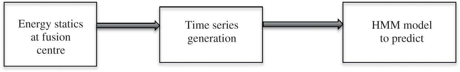
Figure 3: Block diagram for prediction of channel condition

gt∈{u1,u2,…ulγt<λul+1…umγt≥λ (32)

where  gt∈u1,u2,…ul represents PU absent and gt ∈ ul+1…um represents PU present. We want to estimate the next state Xt+1of a PU channel state currently at Xt.

2.4.2 Hidden Markov Model for Primary User Channel Condition Forecasting

In the Hidden Markov Model the system outcome is known and state change probabilities are unknown. Let X = {X1,Xt,….XT} represents the hidden state series where Xt ∈ si, i = 1, 2,…K, si represents states of PU can take a value of 0 and 1. The number of hidden states is denoted by K. Assume O = {O1,Ot,….OT} exhibits the observation sequence where Ot ∈ u1,u2,…uM and a number of the observations is mentioned as M. The transition and the emission probabilities matrix respectively are A and B also the initial state probability vector is represented by π. HMM is represented as θ =  (π, A, B) and considered two unknown states i = 2, π=(π1,π2) is used for calculating above matrices.

A = (aij)K×K (33)

aij=P(Xt+1=sj|Xt=si) (34)

where aij is the probability that for the present state si, the next state is sj. The emission probabilities matrix is given as

B = (bjm)K×M (35)

bjm=P(Ot=uM|Xt=sj)j=1 to K, m=1 to M (36)

here bjm denotes probability for current observation uM, the current state is sj. Let the probability of state series t which ends at state i be

δt(i)=maxX1,…,Xt−1⁡P(X1,…,Xt−1=si;O1,Ot|θ) (37)

To maximize Eq. (37) we use a vector φt(i) which stores the argument values. Following are the steps used in the Viterbi Algorithm to estimate the channel state.

Step 1: Initializes δt (i) and φt (i)

δt(i)=πibi(O1) (38)

φt(i)=0i=1,…,K (39)

Step 2: Repeats to upgrade δt(i) and φt(i)

δt(j)=max1≤i≤K⁡[δt−1(i)aij]bj(Ot)j=1, … K; t = 2, …,T (40)

φt(j)=argmax1≤i≤K⁡[δt−1(i)aij]j=1, … K; t=2, …,T (41)

Step 3: Computes the likelihood probability P*, then estimated state qT∗ by

P∗= max1≤i≤K⁡[δT(i)] (42)

qT∗=argmax1≤i≤K⁡[δT(i)] (43)

to obtain HMM parameters  θ=(π,A,B) statistically Baum-Welch Algorithm and maximum likelihood estimation is used. This estimation is done these ways.

Step 1: Obtain the training observation vectors O1,O2Ot,….OL with length L

Step 2: Obtain θ(1) when k = 1 and update k = k + 1

Step 3: Calculate θ(k) based on O1,O2Ot,….OL. Let the probability of current state si be γt(i) and its transition to next state sj be ζt(i, j)

γt(i)=P(Xt=si|O1,..,OL,θ)t=1, 2 …L (44)

ζt(i,j)= P(Xt=si;Xt+1=sj|OO1,..,OL,θ) (45)

Step 4: Obtain expected values of state si and its transitions to sj as E(γt(i)) and E(ζt(i, j))

E(γt(i))=∑t=1L−1⁡γt(i) (46)

E(ζt(i,j)) = ∑t=1L−1⁡ζt(i,j)  (47)

the parameters calculation from the training sequence in [21] is used.

πi=γ1(i)for i = 1, 2, 3 …K ,at t = 1 (48)

Calculate aij^ by varying i and j from 1 to K

aij^=Expected number of transitions from state si to state sjExpected number of transitions from state si= = ∑t=1L−1⁡ζt(i,j) ∑t=1L−1⁡γt(i) (49)

Calculate bi^(m) by varying i from 1 to K

bi^(m)=Expected number of times in state sj and observing umExpected number of times in state sj=∑t=1Ot=umL⁡γt(i)∑t=1L⁡γt(i) (50)

Step 5: Get the new approximation of aij^ , bi(k) and πi then label it as θ(k + 1)

Step 6: If not converging then go to step 3.

3  Results and Discussions

We assume that PU and SUs are stationary. In our scenario, we considered two PUs and seven co-operative SUs. The simulation is carried out with the assumption of the following parameters as shown in Tab. 1.

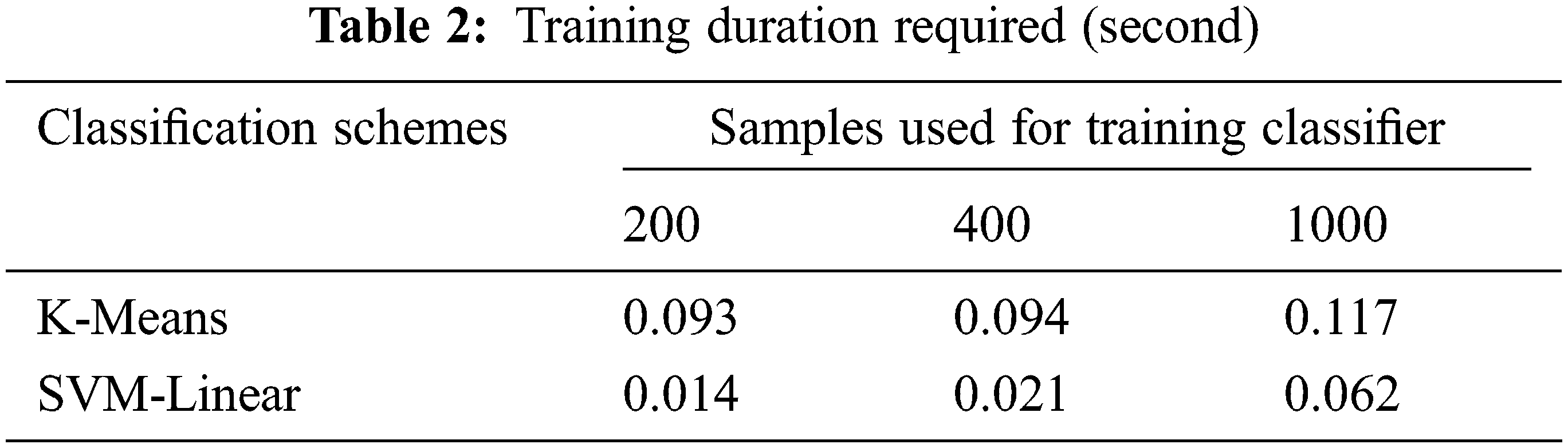
3.1 Training Duration of Classifiers

500 energy vectors were chosen for training each classifier. For unsupervised learning details about channel availability are not required while for supervised learning the channel availability states are required for training. It involves dividing the vectors into clusters and its centroid calculation is done in K-means clustering. But in SVM, locating the hyper-plane which splits the training energy vectors distinctly is the primary task. After successful training of the classifier is completed, the test energy vector is provided for classification. The training duration of classifiers for the size of the energy vector is used for training is shown in Tab. 2. As we increase the number of samples up to 1000 for training the supervised learning technique K-Means technique shows a high training duration (0.117 s) for 1000 samples. Also, the time taken to decide the channel availability is calculated for 1000 samples and obtained as 1.8 × 10−5 for K-Means and 5.5 × 10−5 for SVM.

3.2 Machine Learning Classification

We represent the scatter plot of energy vectors here. In Fig. 4a the K-means method defines a threshold margin between the energy vector points by calculating centroids and classify them as the channel available and unavailable class. Fig. 4b shows SVM algorithm using Linear kernel separates the energy points based on channel availability and draws a decision boundary to determine the threshold for classification.

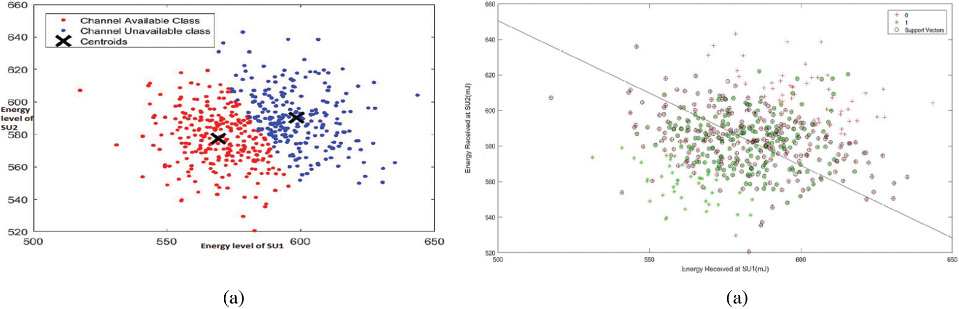
Figure 4: Scatter plot of energy vectors using various classification methods (a) K-Means classification (b) SVM classification

We consider SUs located at different places that are 1 km apart. Fig. 5 presents various CSS methods accuracy in terms of Receiver Operating Characteristic (ROC) curves. It portrays that SVM method is better than the other methods. So this method is suited for multiple primary user cases with high accuracy. The SVM with Linear kernel classifier achieves high detection probability even in the presence of seven secondary users. Also, the unsupervised learning K-Means method is having a comparable performance with the SVM method. By bringing intelligence to the system upgrades the classification process. Even though complexity is associated with SVM, the CR scenario is more prone to lose connectivity the supervised learning is more suitable. AND and OR methods will not produce exact outcomes since outcome depends on all and one decision by CRs.

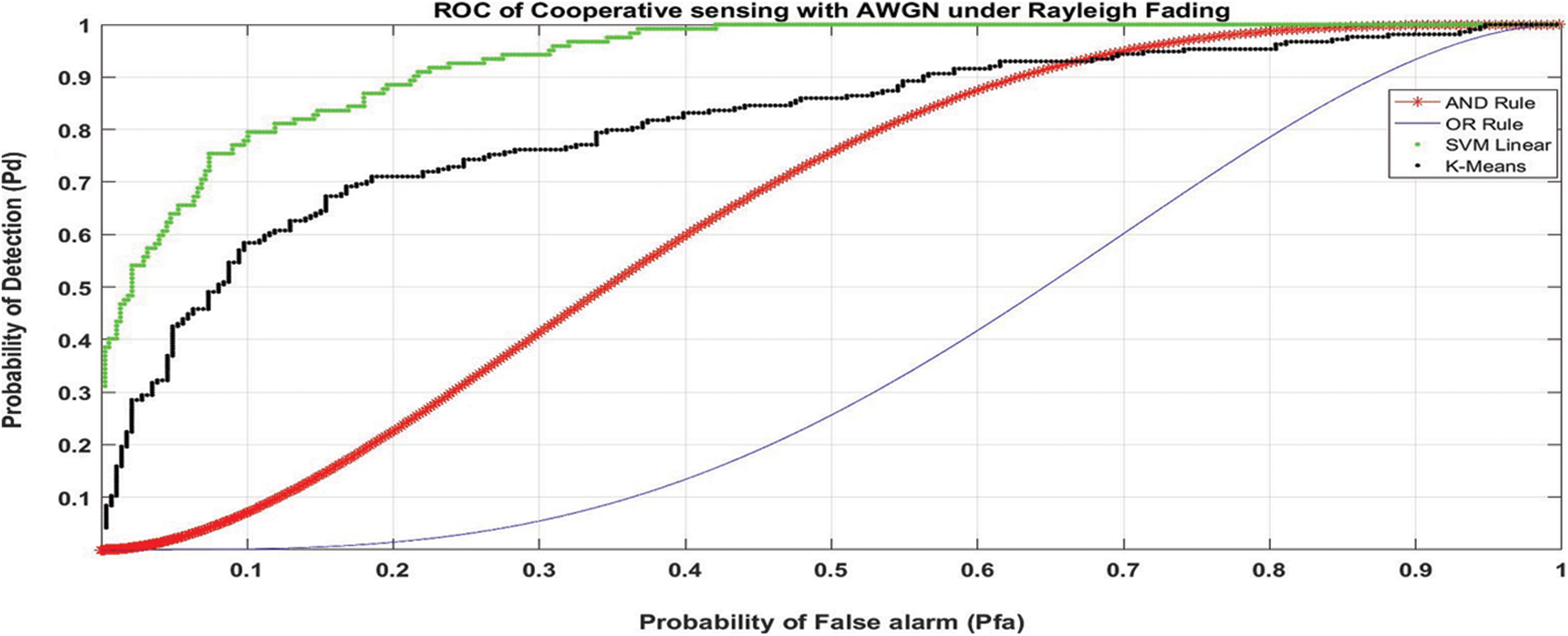
Figure 5: ROC curve of different cooperative spectrum sensing methods

3.3 Numerical Analysis of Spectrum Sensing Using Multiple CR

Numerical outcomes for decision fusion methods are illustrated here. The average snr γ¯ is assumed to be 15 dB. Fig. 6 manifests the probability of missed detection (Pmd) vs. the probability of false alarm (Pfa) under several fading scenarios. Fading channels like Rician, Nakagami-m, Hoyt, Weibull and log-normal shadowing are considered with parameters chosen to be K = 3, m = 3, q = 0.25, v = 6, and σ = 5 dB after running simulations. These parameters are found to be optimal values and it is also coinciding with previous literature. Fading introduces missed detection. We also observe v = 2, Weibull fading channel performance is identical to Rayleigh channel. Apparently, Weibull fading shows the best result among all fading models as the slope of the curve drops quickly. To achieve a Pmd of 1% in a Rayleigh channel, Pfa is found to be 0.8 while in the Weibull channel to obtain the same Pmd, Pfa of even lesser value is obtained, which is highly desirable. It is observed that Pmd value reduces as Pfa increases, hence increase detection probability Pd. This reduction in false alarm probability is required in cognitive radar applications to increase detection probability in cluttered environment. So spectrum utilization can be enhanced. From Fig. 7 it is understood that the probability of detection Pd of 75% is achieved even for very less Pfa in the Weibull fading model when compared with the Rayleigh model which can produce upto 55% only.

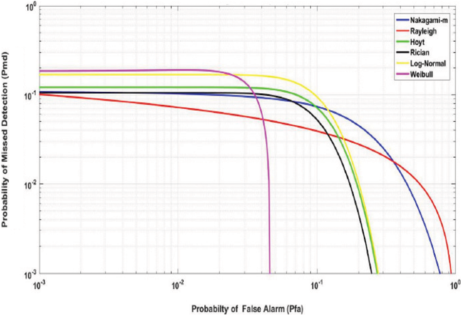
Figure 6: Impact of CR sensing in different fading channels

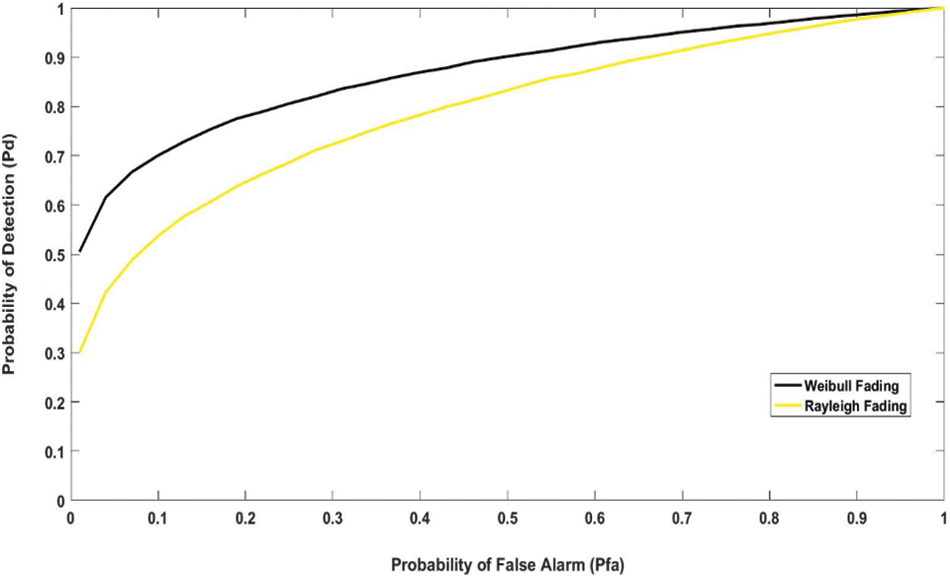
Figure 7: ROC curve for Rayleigh and Weibull fading models (Pd vs. Pfa)

As the Weibull Fading has shown better performance, we utilize this to improve the channel sensing and the fusion decision approach of the cognitive radio network. The Weibull fading has followed a chi-square distribution function. Fig. 8 represents ROC of various decision fusion methods. We consider seven cooperative nodes and for soft fusion rules the assumed SNR values vary from −25 to −15 dB.

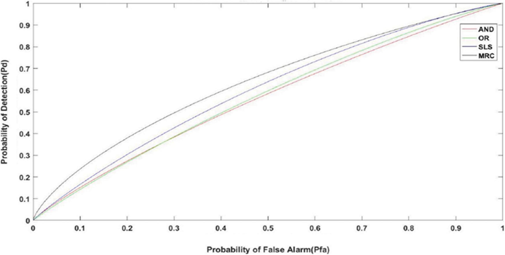
Figure 8: ROC curves for various fusion rules

We keep the probability of false alarm also low. It is evident that MRC outperforms the other schemes. It is due to the right selection of fading channels and learning methods. Detection is done with greater accuracy because the weight vector is chosen optimally. It is achieving a Pd of 70% for a Pfa of 0.5. Even in less SNR, it works well.

Once the energy vectors are obtained they are classified as the channel available and unavailable classes and the SVM-Linear algorithm is used for the classification. The ROC plot shows that the performance of the decision Rules is highly improved and almost reached an accuracy of ∼100% in Fig. 9. MRC reaches the best accuracy of 99.9% where the AND rule has the least accuracy of 97.8%. Over thousand frames this SVM method predicted efficiently when various thresholds are fed into the classifier. The true positive rate obtained for various methods is shown here. Hence it is evident that the Weibull fading along with Chi-Square Distribution has increased spectrum sensing and SVM classifier with MRC can classify the channels with great accuracy. We use 1000 testing frames for classification. Fig. 10 shows thresholds of the above rules is fed into SVM classifier and it achieves detection rate of 99.9%. It depicts the identification of holes in the spectrum which can be effectively utilized. Among various methods, MRC is showing the best performance.

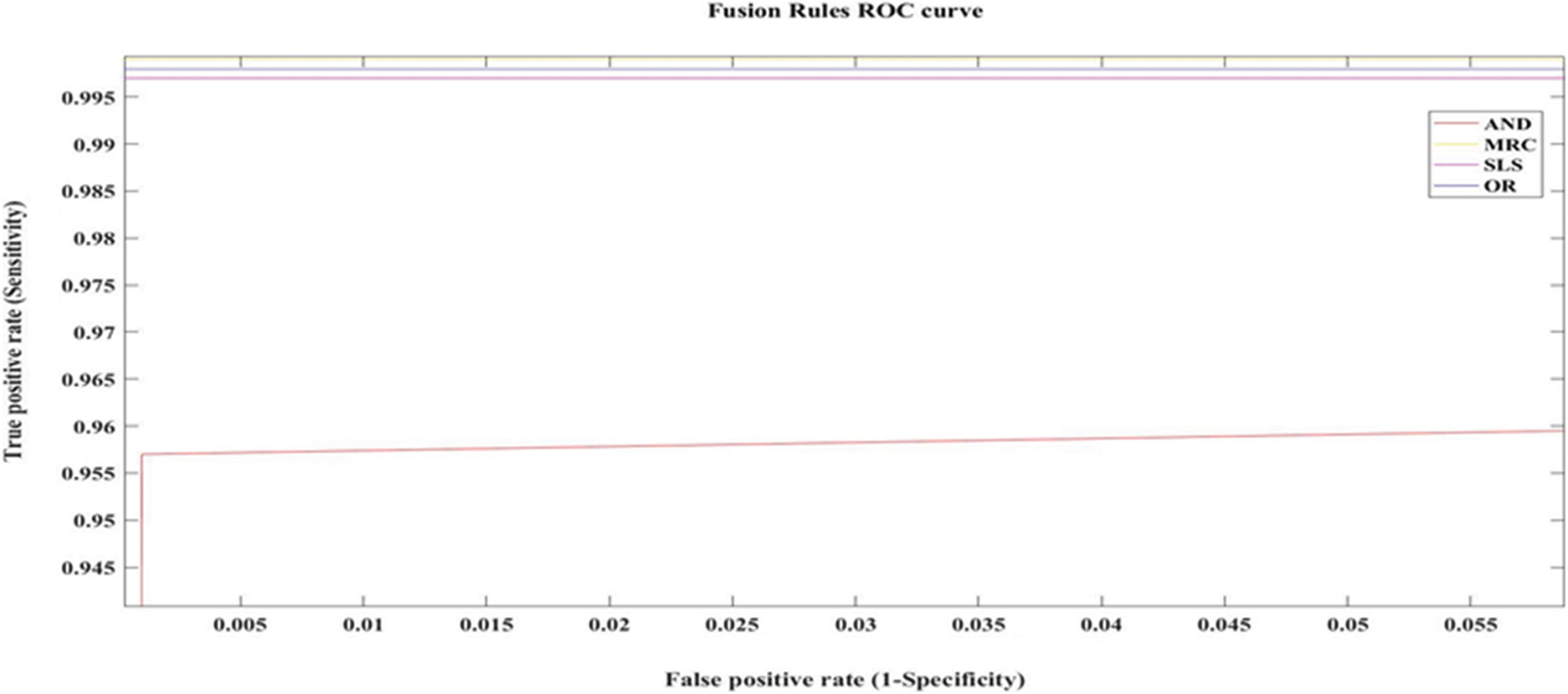
Figure 9: SVM classifier model predicts the output for various fusion thresholds

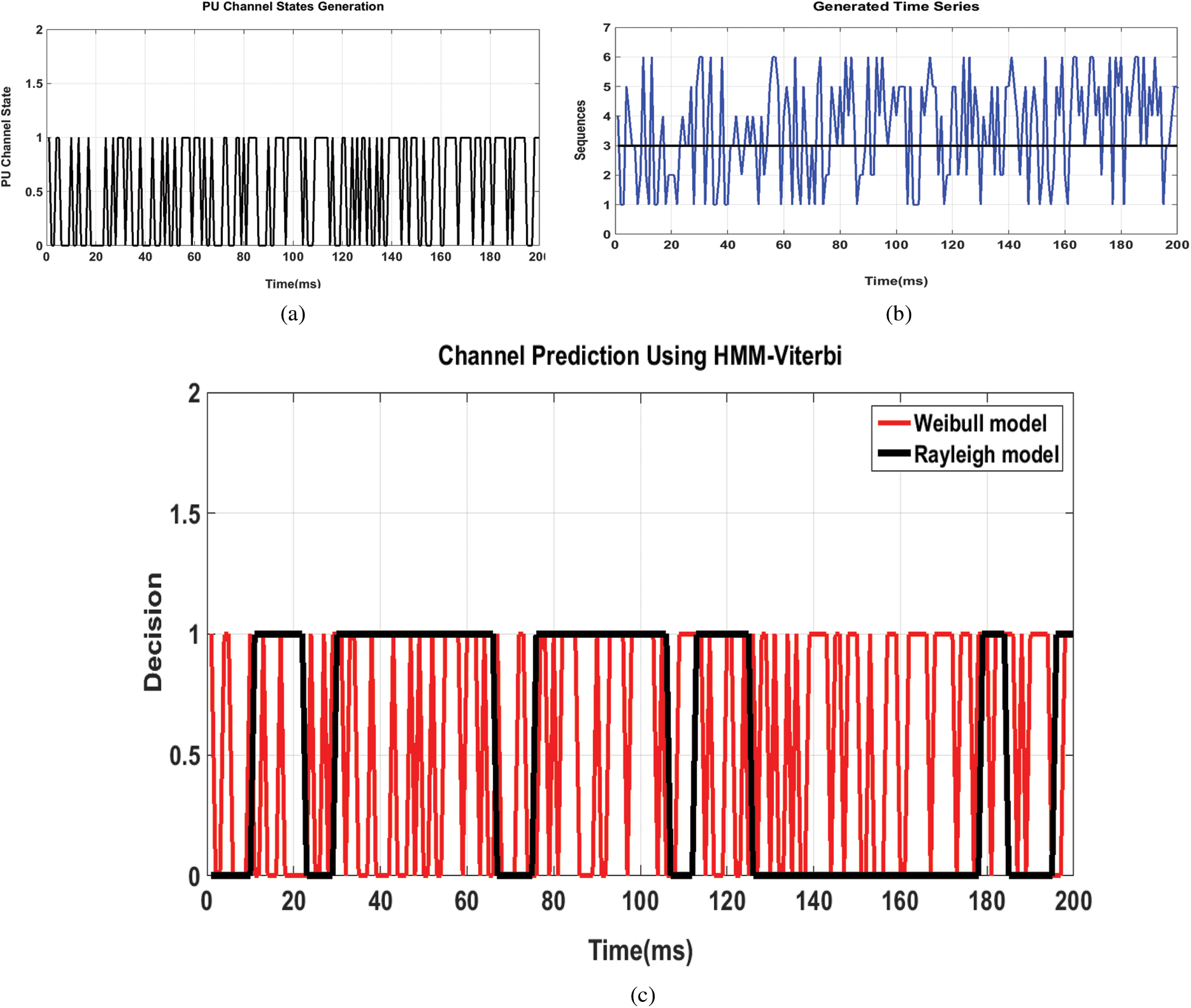
Figure 10: HMM algorithm to capture PU channel conditions (a) Generation of channel states of PU (b) Time series generated for prediction (c) Channel vacancy prediction for various channel models

3.4 Prediction of Primary User Channel State Using HMM Model

To estimate the next state of PU we examine a method and is divided into three steps. First, we find the PU channel state then obtain a model based on the detection that creates a time series to learn about its present condition and finally propose a model for predicting its next state using HMM. For a time period, T = 200 ms Fig. 10a represents the random distribution of PU channel conditions. It presents the state of the PU in a particular channel. It has both idle state (channel available state) and occupied state (channel unavailable state). These idle states are termed as the spectrum holes and can be effectively used for the SU communication in CRN. In Fig. 10b to differentiate the state of activity of the PU channel a margin is drawn. The points below the margin show the amount of the spectrum holes in a channel. While the points above the margin show the instances at which the channel is occupied by the PU. This sequenced time series is used as the input parameter for the HMM prediction model. Once the sequenced time series is generated, it is used along with emission and transmission probability for the prediction of the channel. The Hidden Markov Model along with Viterbi and Baum Welsh algorithm is used for the Spectrum Prediction. It is evident that the prediction performance has reached 100% as the result of using the Weibull Fading Model for a period of 200 ms from Fig. 10c when compared to the Rayleigh model which is achieving only 84.5% accuracy in prediction. Hence the spectrum prediction of the PU channel activity is done with maximum accuracy.

4  Conclusion

Thus an efficient machine learning algorithm for spectrum sensing and prediction is developed and simulated in the wireless cognitive environment. The spectrum sensing was initially done with the Rayleigh fading model and the channel was classified with the help of machine learning but it has shown a poor act in terms of detection. Hence an improvisation by considering the other channel fading models and tested them in the wireless environment is found. As a result, the Weibull fading model is the best fading model to use in both indoor and outdoor wireless environments. Further to find the best fusion rule algorithm to suit this scenario, we conducted the performance comparison of soft and hard fusion rules and found maximal ratio combining algorithm is performing well by making use of receiver diversity in multiple CRs. Thus we combined the Weibull fading model with the MRC fusion rule and tested it in the cognitive environment under the chi-square distribution for multiple secondary users and this resulted in better detection characteristics. Then HMM with Baum Welsh and Viterbi Algorithm is used for the spectrum prediction by generating a time series to capture the states of PU. This has given a high accuracy in forecasting the next state of the channel.

The chosen energy vectors correctly train the classifier to find the occupancy of the primary user. The duration of training is found to be very less. So SVM method can be a good choice to get a decision on the channel conditions ambiguity. Among various fading models, the Rayleigh model is due to multipath reception and all the other models are its variants. By doing simulations we obtain the best possible values of severity factor of all the methods and found out that detection is good in the Weibull method. It is observed that the Pmd value reduces as Pfa increases, hence increase detection probability. This reduction in missed detection is required in cognitive radar applications to identify targets in a cluttered environment. Thus spectrum utilization can be enhanced. The simulation results revealed that the classifier trained with the ML algorithm helps the fusion center to attain well in terms of sensing accuracy. From the received statistics MRC method gives its best because of the accurate choice of weight parameter based on energy data obtained from all CR users. The fusion center can conclude channel status accurately. Then Hidden Markov model is used to study the occupancy of the primary user channel and predicts its near future to make use of spectrum is efficiently and found out that high accuracy in predicting the occupancy of the channel. Using this model the prediction in various fading models is done and found out that using time series-forecasting model completely fits on past data and using them to predict future interpretation. This work finds application in the field of 5G technology where the wireless spectrum is very important to be shared with lots of IoT machines and smart devices for communication.

Funding Statement: The authors received no specific funding for this study.

Conflicts of Interest: The authors declare that they have no conflicts of interest to report regarding the present study.

This work is licensed under a Creative Commons Attribution 4.0 International License, which permits unrestricted use, distribution, and reproduction in any medium, provided the original work is properly cited.