DOI:10.32604/iasc.2022.024310
| Intelligent Automation & Soft Computing DOI:10.32604/iasc.2022.024310 | |
| Article |
MLP-PSO Framework with Dynamic Network Tuning for Traffic Flow Forecasting
1Department of Computer Science and Engineering, Sri Venkateswara College of Engineering, Sriperumbudur, India
2Department of Electronics and Communication Engineering, Sri Venkateswara College of Engineering, Sriperumbudur, India
*Corresponding Author: V. Rajalakshmi. Email: vraji@svce.ac.in
Received: 13 October 2021; Accepted: 13 December 2021
Abstract: Traffic flow forecasting is the need of the hour requirement in Intelligent Transportation Systems (ITS). Various Artificial Intelligence Frameworks and Machine Learning Models are incorporated in today’s ITS to enhance forecasting. Tuning the model parameters play a vital role in designing an efficient model to improve the reliability of forecasting. Hence, the primary objective of this research is to propose a novel hybrid framework to tune the parameters of Multilayer Perceptron (MLP) using the Swarm Intelligence technique called Particle Swarm Optimization (PSO). The proposed MLP-PSO framework is designed to adjust the weights and bias parameters of MLP dynamically using PSO in order to optimize the network performance of MLP. PSO continuously monitors the gradient loss of MLP network while forecasting the traffic flow. The loss is reduced gradually using Inertia Weight (denoted as ω) which is the critical parameter of PSO. It is used to set a balance between the local and global search possibilities. The Inertia Weight has been varied in order to dynamically adjusts the network parameters of MLP. A comparison has been carried out among MLP and MLP-PSO models with variants of Inertia Weight Initializations. The results obtained justifies that, the proposed MLP-PSO framework reduces the forecasting error and improves reliability and accuracy than MLP model.
Keywords: Multilayer perceptron; evolutionary computing; particle swarm optimization; swarm intelligence; forecasting
There are rapid advances in Intelligent Transportation Systems (ITS) due to its high potential to improve safety and mobility in transportation. The main motivation behind the implementation of ITS is the effective and efficient forecasting of traffic flow on roads thus facilitating a safer and smarter use of traffic networks. The implementation of such systems aims in forecasting with negligible error rates. A traffic flow forecasted from multilayer perceptron output depends on the input and parameters of the network. The performance of the network can be optimized by Bio-inspired computer optimization algorithms.
Bio-inspired computer optimization algorithms are a novel way to developing new and robust competing approaches that is based on the ideas and inspiration of biological evolution. In recent years, bio-inspired optimization algorithms have gained popularity in machine learning for solving challenging issues in science and engineering. However, these problems are typically nonlinear and constrained by many nonlinear constraints in determining the best solution. Recent advances tend to utilize bio-inspired optimization algorithms to solve the issues of traditional optimization methods, which provide a potential technique for solving complex optimization problems.
Various population-based nature inspired metaheuristic optimization algorithms are used with the Machine learning models in order to train the parameters of the model. Some of the algorithms used are Ant Colony optimization (ACO) [1], Particle swarm optimization (PSO), Firefly Algorithm (FA) [2], Moth flame Optimization (MFO), Chicken Swarm Optimization (CSO) [3], Elephant Herding Optimization (EHO) [4], Cuckoo Search (CS) [5] etc.
Particle Swarm Optimization (PSO) is utilized in this study to improve the performance of the Multilayer Perceptron and to find the optimal solution for forecasting traffic flow. With this forecasting model the error rate is reduced and hence the prediction accuracy is improved.
Garg et al. used PSO to train Artificial Neural Network (ANN) for drilling flank wear detection. The network parameters are tuned using the PSO. The results show that the PSO trained ANN performs much better than Back Propogation Neural Network (BPNN).
The main feature of PSO is to provide minimum velocity constraint. This feature avoids premature convergence in MLP network parameter tuning. It also reduces the impact of increasing the dimensions of MLP. These improvements in network tuning [6] provides reduced error rate in prediction as stated by Pu et al.
A combined scheme using PSO and Newton’s law of motion named as centripetal accelerated particle swarm optimization (CAPSO) was proposed by Beheshti et al. CAPSO is applied to MLP to optimize the network parameters. The CAPSO applied on MLP was able to classify diseases in various medical datasets efficiently that the nature inspired algorithms such as PSO [7], imperialist competitive algorithm and GSA on MLP.
Dang et al. applied PSO and Firefly algorithms to ANN to estimate the scour depths. The result prove Firefly [8] on ANN was effective compared to PSO on ANN. Guofeng Zhou et al. applied Artificial Bee Colony (ABC) Optimization and Particle Swarm Optimization (PSO) on MLP for estimating the usage of heating and cooling loads of the energy in the residance. The R2, MAE and RMSE metrics are used to measure the performance of the models. The results show that PSO on MLP works efficient than ABC on MLP [9].
Multimean particle swarm optimization is a novel optimization approach introduced by Mehmet et al. This algorithm was used to train a multilayer feed-forward ANN. On multilayer feed-forward ANN training, the technique was found to generate superior results than multiple swarm optimization (MSO) on benchmark datasets [10].
In cognitive research, the acquired data for training contains uncertain information. This uncertain data is termed as fuzziness. Training the MLP with this fuzzy data is called as Fuzzy MLP model [11] by Dash et al. MLP normally suffers from local minima problem. To overcome this, three metaheuristic algorithms particle swarm optimization, genetic algorithm and gravitational search are used to optimize the parameters of FMLP.
To optimize the operation of the thermal producing units, Thang et al. suggested an updated firefly method. At various levels, three fundamental modifications to the firefly algorithms were presented. The improved algorithm was applied on the five different benchmarks and attained better performance than the firefly algorithm [12].
Khatibi et al. proposed hybrid algorithms. One is MLP with Levenberg–Marquardt (LM) backpropagation algorithm [13] and the other is MLP with Fire-Fly Algorithm. These algorithms were used to predict the directions of stream flow and the result show MLP with Fire-Fly Algorithm performs better.
Emad et al. use the swarm intelligence Firefly method as a classifier. The suggested technique has three stages [14]. The first stage is feature selection, the second stage is model construction using FA to classify the class labels and the last stage is prediction of the classes. The classifier performance was proved to be effective by applying to seven different datasets.
Aboul et al. [15] employed Moth flame optimization to optimize the parameters of the support vector machine in detecting tomato diseases. The fitness function in MFO captures the dependency in the features more efficiently and thereby maximized the classification accuracy. Xiaodong et al. proposed a modified Ameliorated Moth Flame Optimization (AMFO) algorithm [16] in which the flames are produced with Gaussian mutation and thereby the moth postions are updated. This enables the MFO to attain the global minimum faster. On 23 separate benchmarks, this algorithm was compared to 9 state-of-the-art models and achieved good results with 0.0542 mean square error.
The hybrid algorithm combining the Deep Neural Network and Chicken Swarm Optimization is proposed by [17] Sengar et al. The DNN was initially trained with 24 h wind energy data. The error rate during training the DNN model is reduced using CSO. Later the wind energy forecast was carried out using the DNN-CSO algorithm. This algorithm showed better performance when compared with DNN and ANN models.
Saghatforoush et al. predicted the flyrock and back break in order to minimize the environmental impacts due to back break, flyrock and ground vibration [18]. The Artificial Neural Network (ANN) algorithm was used in flyrock and back break prediction. In order to increase prediction accuracy, the parameters of the ANN were fine-tuned effectively utilising Ant Colony Optimization (ACO).
Hossein et al. presented a hybrid approach that combines elephant herding optimization (EHO) and MLP [19] to optimize the cooling loads in heating, ventilation, and air conditioning. ACO with MLP and Harris hawks optimization (HHO) with MLP were used to compare the outcomes. The proposed EHO with MLP outperformed the other two metaheuristic algorithms in terms of accuracy.
The performances of Feed forward neural networks was improved by optimizing its parameters. In this paper, Ashraf et al. [20] compared the effectiveness of various single objective and multi objective optimization algorithms. AbdElRahman et al. proposed a strategy to refine the cell structure of Long Short Term Memory (LSTM) Reccurent Neural Networks (RNN) using Ant Colony Optimization (ACO) [21]. The ACO optimized LSTM RNNs performed better than the traditional algorithms.
A simple matching-grasshopper new cat swarm optimization algorithm (SM-GNCSOA) was proposed by [22] Bansal et al. in order to select the relevant featyres efficiently. It was used to optimize the performance of Multilayer Perceptron (MLP). This gives better results when applied to various datasets and very efficient to avoid local minima problems. Monalisa et al. used Elephant Herding Optimization algorithm [23] for tuning the network parameters of ANN. This resulted in diagnosis of cancer with good classification accuracy of about 0.9837.
One of the most important topics in Particle Swarm Optimization (PSO) [24] is determining the inertia weight w. The inertia weight was created by PSO to balance its global and local search capabilities. Initially, a method was proposed for adjusting the inertia weight adaptively based on particle velocity data. Second, Zheng et al. propose that both position and velocity data be used to adaptively modify the inertia weight.
Martins et al. developed the linear decreasing inertia weight (LDIW) technique [25] to increase the performance of the initial particle swarm optimization. However, when dealing with big optimization problems, the linear decreasing inertia weight PSO (LDIW-PSO) algorithm is known to have the defect of premature convergence due to a lack of momentum for particles to execute exploitation as the programme approaches completion.
Particle swarm optimization (PSO) is a well-known swarm intelligence-based optimization technique [26]. PSO’s inertia weight is a crucial parameter. During the last 20 years, many methodologies for determining inertia weight have been proposed by Kushwah et al. This study proposes a Dynamic Inertia Weight method. In the suggested method, probability-based inertia weights are applied to PSO. This paper demonstrates the potential of particle swarm optimization for tackling many types of optimization problems in chemometrics by providing a full description of the method [27] as well as several worked examples in diverse applications is proposed by Marini et al.
Shang et al. present a novel hybrid prediction model based on combination kernel function-least squares support vector machine and multivariate phase space reconstruction [28] to increase traffic prediction accuracy. PSO is used to optimize the parameters of the given model. Cong et al. proved that the least squares support vector machine (LSSVM) [29] has a lot of potential in forecasting issues, particularly when it comes to selecting the values of its two parameters using appropriate heuristic approaches. However, the difficulty in understanding and obtaining the global optimal solution with these meta-heuristics. The fruit fly optimization algorithm (FOA) is a novel heuristic method that is easy to learn and quickly converges to the global optimal solution.
An upgraded PSO-BP (particle swarm optimization-back propagation) prediction model is built to estimate total vessel traffic flow in a particular port location. The SAPSO-BP neural network is a prediction model presented by Zhang et al. [30] that updates the parameters of a BP neural network using the SAPSO (self-adaptive particle swarm optimization) algorithm.
In this work, the researcher’s ideas motivated in optimizing the performance of MLP using Particle Swarm Optimization.
3 Multilayer Perceptron (MLP) Framework
Multilayer Perceptron is a fully connected feedforward back propagation network. There can be three or more layers consisting of an input layer, an output layer and one or more hidden layers forming a deep neural network. In a fully connected network, the node in one layer connects to every node in the next layer with a certain weight w. The model is trained by changing the connection weights after each iteration based on the amount of error in the output. Figs. 1 and 2 shows the MLP framework and the weight and bias initialization.
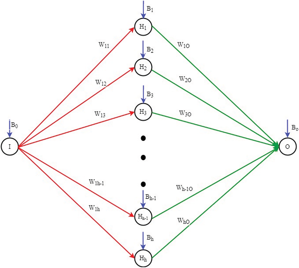
Figure 1: Multilayer perceptron
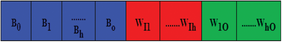
Figure 2: Bias and weights representation in MLP

Figure 3: MLP-PSO framework for traffic flow forecasting
Algorithm 1 is an implementation of multilayer perceptron with backpropogation for time series forecasting. X, Y are the input and the target time series data points which is fed as input data to multilayer perceptron algorithm. Initialize the two main parameters in perceptron algorithm namely: the learning rate (η) and the number of times to perform back propagation (epoch). Later, initialize the following:
• Wh-weight between the input layer and hidden layer
• Wout-weight between the hidden layer and output layer
• Bh-bias to hidden layer neurons
• Bout-bias to output layer neurons
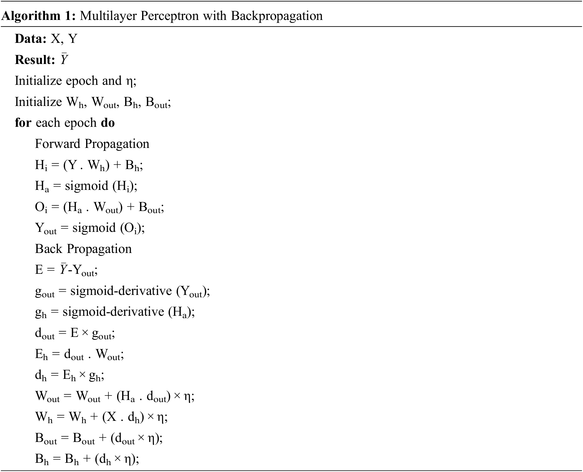
The following are computed for forward propagation:
1. Hidden layer input (Hi) which is the dot product of Y and Wh added to Bh
2. Hidden layer activation (Ha) obtained by applying sigmoid activation function to Hi
3. Output layer input (Oi) which is the dot product of Ha with Wout added to Bout
4. Predicted output (Yout) obtained by applying sigmoid activation function to Oi
After forward propagation, an output is predicted which may contain error. In order to minimize the error rate, the network is back propagated by updating the weights and bias at all intermediate layers between output and input layer. The following computations are done in backward propagation:
1. Error (E) which is the difference between original output (
2. Slope or gradient of output layer (gout) and hidden layer (gout) which are obtained by applying derivative of sigmoid function to Yout and Ha respectively.
3. Delta of the output layer (dout) is the product of E and gout
4. Error in hidden layer (Eh) is the dot product of dout and Wout
5. Delta of the hidden layer (dh) is the product of Eh and gh
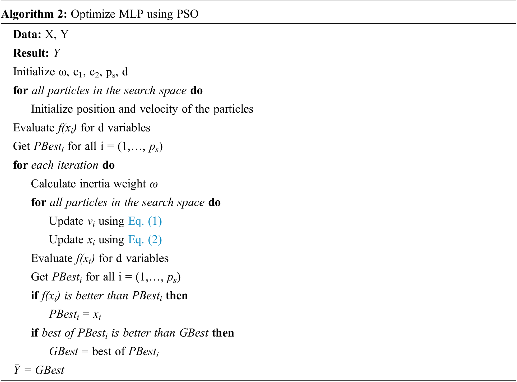
Particle Swarm Optimization (PSO) is a meta-heuristic optimization technique based on natural swarm behaviour, such as fish and bird schools. PSO is a simple social system simulation. The PSO algorithm was created with the goal of graphically simulating the elegant but unpredictable choreography of a flock of birds.
Each solution in PSO is a “bird” with in problem space which is known as “particle”. All particles have fitness values that are evaluated by the fitness function in order to be optimized, as well as velocities that direct the particles’ flight. The particles follow the current optimum particles through the search space.
This technique is a basic yet effective population-based, adaptive, and stochastic technique for tackling simple and challenging optimization problems. Because it does not require the gradient of the problems to work with, the technique can be used to a wide range of optimization problems. In PSO, a swarm of particles (a collection of solutions) is scattered at random across the search space. The food at each particle’s location is specified by the target function (which is the value of the objective function). Every particle is aware of its initialization value, best value (locally best solution), swarm-wide best value (globally best solution), and velocity as determined by the objective function.
A single static population is maintained by PSO whose particles are slightly adjusted due to variations in search space. This method is referred as directed mutation. These particles never expire instead moved to different space due to directed mutation.
A small number of different parameters, such as the number of particles in the swarm, the dimension of the search space, the particle’s velocity and position, cognitive rate, social rate, inertia weight and other random factors, control the PSO algorithm’s behaviour and usefulness in optimizing a given problem. The versatility of PSO lies in tuning these parameters for optimal solution. To be more specific, handling inertia weight has attracted many researchers’ interest. This is due to the fact that the parameter ω controls the divergence or convergence of particles. The position and velocity in a d dimensional space of the particles are represented by xi = xi1, xid and vi = vi1, . . . vid respectively. Particle movement is required to find the best solution in the search space.
PSO starts with a set of random particles (solutions) and then updates generations to look for optima. Each particle is updated in each iteration by comparing two “best” values. The first is the best solution (fitness) obtained by the particle thus far which is called as PBest. The best value obtained so far by any particle in the population is another “best” value recorded by the particle swarm optimizer. This best value is referred to as GBest, which stands for “global best”.
Consider the following notations:
• f-MLP function to optimize
• ps-number of particles in the swarm
• d-dimension of the search space
• c1-cognitive coefficient
• c2-social coefficient
• ω-inertia
• vi-velocity of the ith particle
• xi-position of the ith particle
• PBesti-local best solution of the ith particle
• GBest-global best among other particles in the swarm
• r1 and r2-random values obtained from rand() function
For the next iteration, the velocity and position of the particles are updated as
Fig. 3 shows the proposed MLP-PSO framework for traffic flow forecasting. The objective of MLP-PSO framework is to minimize the error rate compared to MLP. Hence, the objective function of PSO is to minimize the Mean Square Error (MSE).
4.1 Parameter Selection in PSO
The inertia, cognitive coefficient and social coefficient are the parameters that control the behaviour of the swarms. At each iteration, the random terms are used to accelerate the cognitive and social behavior. The weights r1 and r2 are used to stochastically adjust the cognitive and social acceleration respectively. r1 and r2 are unique for each iteration and each particle. They are random values set in the range of [0, 1].
The c1 and c2 parameters defines the group’s capability to experience the best personal solutions and the best global solution found over the iterations respectively. When c1 is high, there is no convergence since each particle is focused on its own best solutions. When c2 is high, the optimal solution cannot be reached. Most of the studies states that c1 + c2 > 4.
For N iterations and for every i current iteration, c2 linearly increases from 0.5 to 3.5 whereas c1 linearly decreases from 3.5 to 0.5. This ensures c1 + c2 = 4 [25].
4.2 Variants of Inertia Weight (ω)
Particles’ ability to identify the best solutions found so far is known as exploitation. Particles’ ability to evaluate the entire search space is referred to as exploration. A good balance on exploitation and exploration likely has an impact on the convergence to optimum solution. The inertia weight is a critical parameter in the PSO process, since it influences convergence and the trade-off between exploration-exploitation. Some variants of inertia weights are used that shows its impact on the forecasted traffic flows. Various studies states that ω can be initially 0.9 (referred as ωstart) and converges down to 0.4 (referred as ωend) in the subsequent iterations.
4.2.1 Constant Inertia Weight (CIW)
A constant value is set for the inertia in all iterations. In this work, the constant value is set as
4.2.2 Random Inertia Weight (RIW)
The Random Inertia Weight is fully determined by a random value. The generated random value is in the range [0, 1] and the computed RIW is between [0.4, 0.9]
4.2.3 Chaotic Inertia Weight (ChIW)
A dynamic nonlinear system that is highly dependent on its starting value is called a chaos. It possesses the properties of ergodicity and stochasticity. The goal is to use the merits of chaotic optimization to prevent PSO entering into local optimum in the problem search process.
where zk is the kth chaotic number in the range [0, 1] and μ = 4 such that, z0 ∈ (0, 1) and z0 ∉ (0, 0.25, 0.5, 0.75, 1)
4.2.4 Linear Decreasing Inertia Weight (LDIW)
For every subsequent iteration, the inertia weight decreases linearly. In general, a large inertia weight is advised for the initial phases of the search process to increase global exploration (finding new areas), whereas the inertia weight is reduced for local exploration in the later stages in order to fine tune the current search space. Considering imax and i are maximum and current iterations respectively, the Linear Decreasing Inertia Weight (LDIW) is computed as follows:
5 Experimental Setup and Discussion
In order to have a comprehensive evaluation of the model, three metrics are considered to validate the models. Mean Square Error (MSE) is used to show the degree of variation in the results. Mean Absolute Error(MAE) is used to show the variance in the result prediction. R2 is used to measure the degree of correlation between the original value and the predicted value.
• At-the original traffic flow at time t
• Ā-average of the original traffic flows
• Ft-the predicted traffic flow at time t
• num-number of traffic flow data
Metrics are given by,
Time Series Traffic Flow dataset used in this paper is recorded from MIDAS Site-5825 at M48 westbound between M4 and J1 (102022401)–UK [31]. The traffic flow data comprises of traffic flow data for every 15 min interval of each day for every month. The model is trained and tested with Monday 8 AM data in the year 2020. The data is preprocessed before training to obtain a stationary time series. 44 traffic flow values are available for Mondays in the dataset. In this, 39 data is used to train the models. The forecast for last 5 Mondays in the year 2020 are predicted and tested with various models.
The 1 × 10 × 6 × 1 MLP model is built. The model represents one node at input and output layer, 10 and 6 nodes in the first and second hidden layers respectively. The learning rate η is set as 0.1. After various runs of the algorithm by varying the number of epochs, it has been identified that the gradient loss is minimized at 50 epochs. The weight and bias is initialised at random during the initial run of PSO. Later PSO generates the weight and bias based on the loss from MLP which is stated in Algorithm 2. The position and velocity of the particles are updated in the range 0–1. The size of search space is set as 100. Other parameter setting of PSO is carried out as per the discussion in Section 4.1.
Tab. 1 shows the result of training by various models. While training the models, the MLP-PSO with Linear Decreasing Inertia Weight (LDIW) yields MSE of 0.182, MAE of 0.250 and R2 of 0.981, whereas MLP yields MSE of 0.720, MAE of 0.640 and R2 of 0.882. Testing results of all the models are displayed in Tab. 2. In the same way, during testing the models MLP-PSO (LDIW) yields MSE of 0.148, MAE of 0.240 and R2 of 0.979 and MLP yields MSE of 0.666, MAE of 0.620 and R2 of 0.899. The results show that MLP-PSO with variants of inertia provides better performance than MLP model. Figs. 4–8 shows the comparison of actual and predicted forecast from all the models.
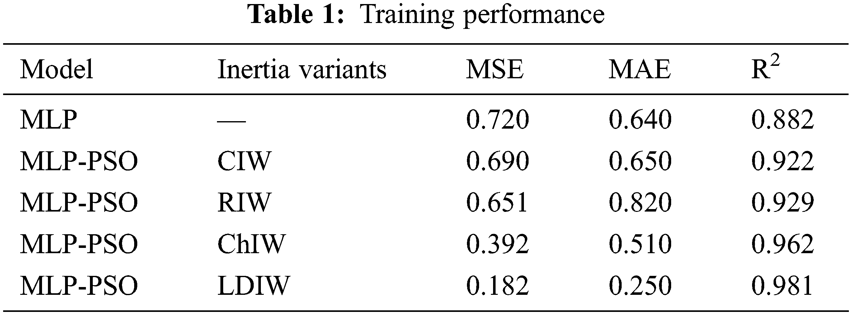
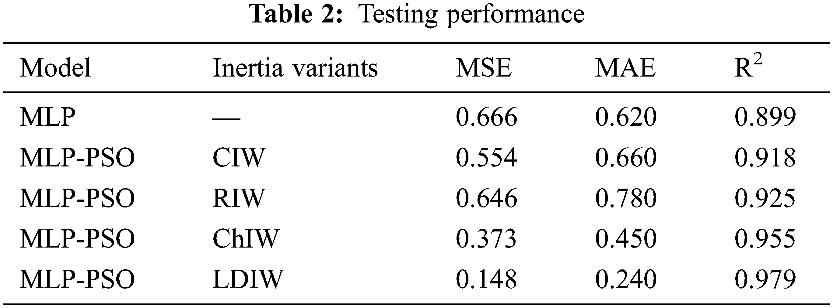
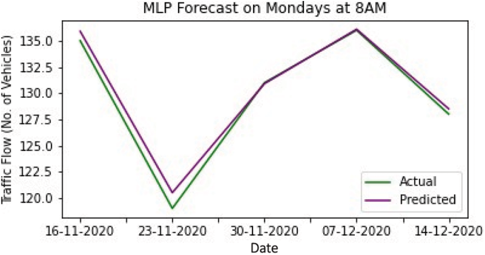
Figure 4: MLP forecast
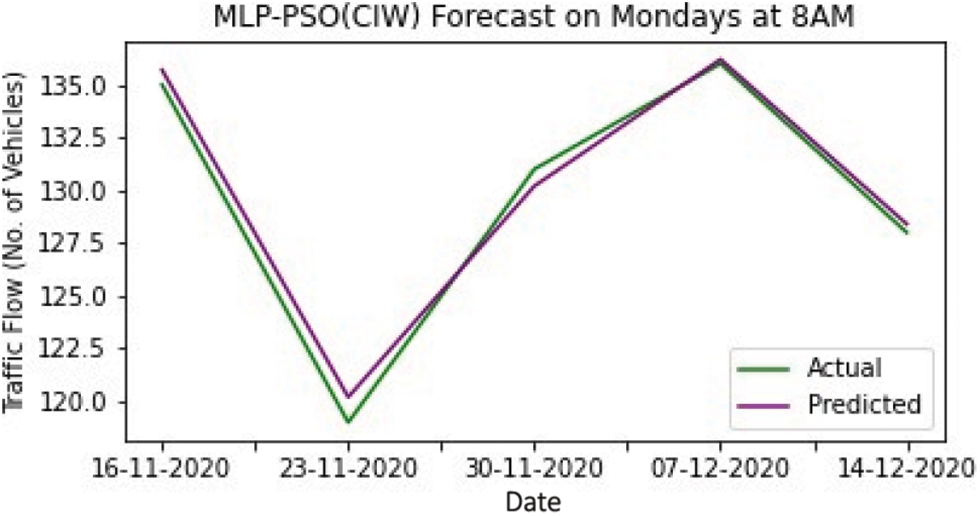
Figure 5: MLP-PSO (CIW) forecast
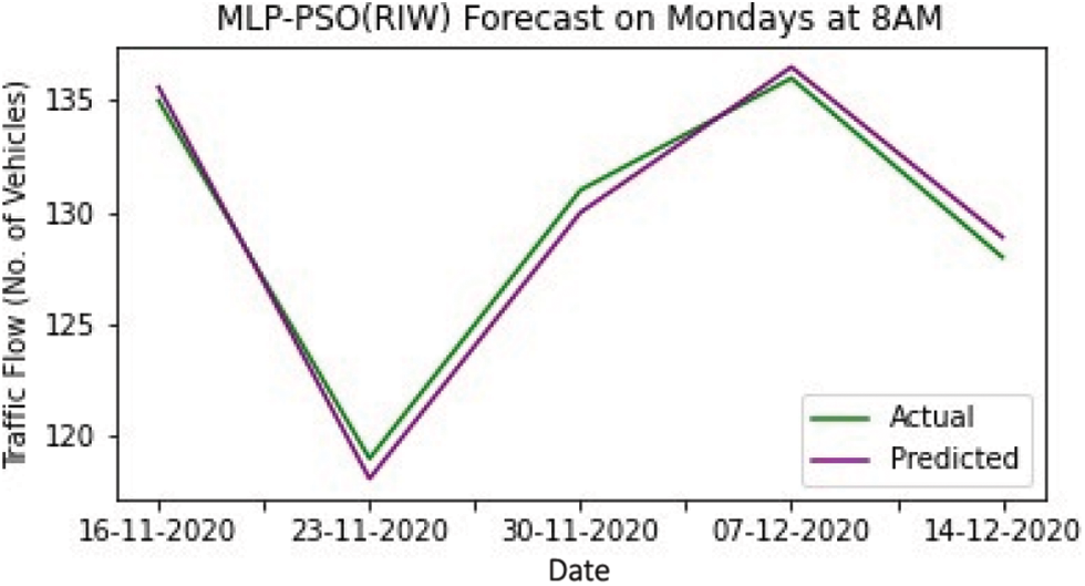
Figure 6: MLP-PSO (RIW) forecast
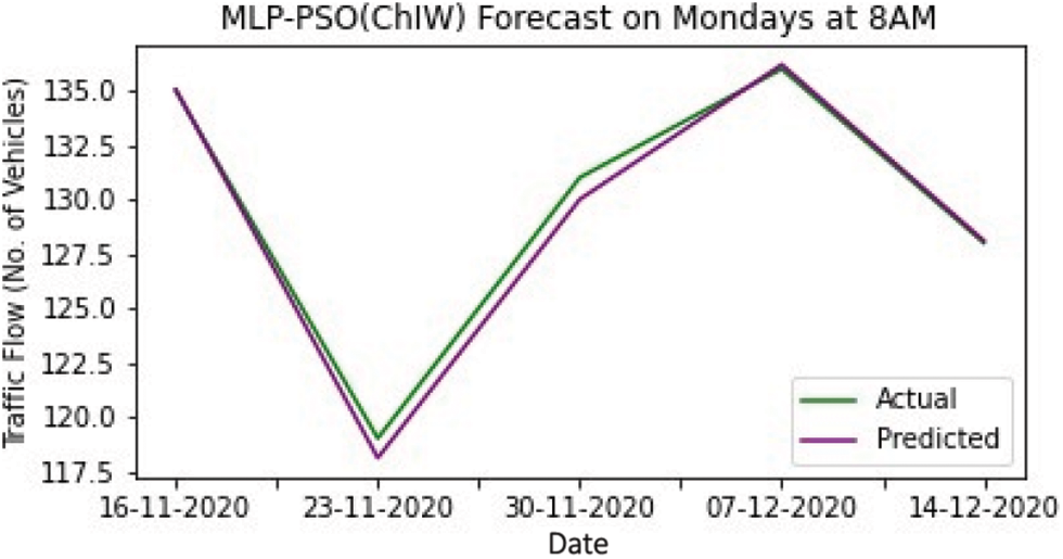
Figure 7: MLP-PSO (ChIW) forecast
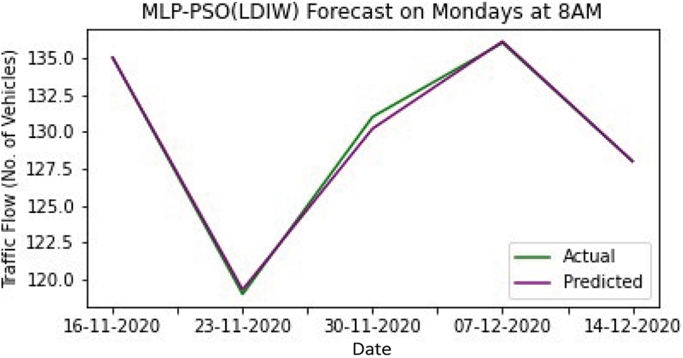
Figure 8: MLP-PSO (LDIW) forecast
Traffic flow forecasting is research of estimating the number of vehicles in the future that may flow through a particular lane at a specified period. The accurate estimation of future traffic flows is quite challenging. Numerous machine learning models are prevalent in the forecasting of time series data. In this paper, a novel approach of optimizing the MLP framework with PSO is proposed. The time series traffic flow data of MIDAS highway is considered for forecasting in this study. The MLP and MLP-PSO models with variants of Inertia Weight initialization are trained and tested to suggest a model with high accuracy. The MLP-PSO with Linear Decreasing Inertia Weight (LDIW) provides better accuracy with Mean Square Error (MSE) of 0.148, Mean Absolute Error (MAE) of 0.240 and R2 of 0.979 compared to MLP with MSE of 0.666, MAE of 0.620 and R2 of 0.899 in testing. Finally, the results obtained shows that MLP-PSO with all variants of Inertia weight provides improved accuracy rate than MLP.
Acknowledgement: We would like to thank our colleagues from our institution for providing deeper insights and expertise that helped our research to great extent.
Funding Statement: The authors received no specific funding for this study.
Conflicts of Interest: The authors declare that they have no conflicts of interest to report regarding the present study.
1. S. Garg, K. Patra and S. K. Pal, “Particle swarm optimization of a neural network model in a machining process,” Sadhana, vol. 39, pp. 533–548, 2014. [Google Scholar]
2. J. Nayak, B. Naik and P. Dinesh, “Firefly algorithm in biomedical and health care,” Advances, Issues and Challenges. SN Computer Science, vol. 1, pp. 311–320, 2020. [Google Scholar]
3. S. Deb, X. Z. Gao and K. Tammi, “Recent studies on chicken swarm optimization algorithm: A review,” Artificial Intelligence Review, vol. 53, pp. 1737–1765, 2020. [Google Scholar]
4. L. Juan, L. Hong, A. H. Alavi and G. Wang, “Elephant herding optimization: Variants, hybrids, and applications,” Mathematics, vol. 8, pp. 1415–1425, 2020. [Google Scholar]
5. A. S. Joshi, K. Omkar, G. M. Kakandika and V. M. Nandedkar, “Cuckoo search optimization-A review,” Materials Today: Proceedings, vol. 4, no. 8, pp. 7262–7269, 2017. [Google Scholar]
6. X. Pu, Z. Fang and Y. Liu, “Multilayer perceptron networks training using particle swarm optimization with minimum velocity constraints,” in Advances in Neural Networks–ISNN 2007. Lecture Notes in Computer Science, Springer, Berlin, Heidelberg, vol. 4493, 2007. [Google Scholar]
7. Z. Beheshti, S. M. H. Shamsuddin and E. Beheshti, “Enhancement of artificial neural network learning using centripetal accelerated particle swarm optimization for medical diseases diagnosis,” Soft Computing, vol. 18, pp. 2253–2270, 2014. [Google Scholar]
8. N. M. Dang, D. Tran Anh and T. D. Dang, “ANN optimized by PSO and firefly algorithms for predicting scour depths around bridge piers,” Engineering with Computers, vol. 37, pp. 293–303, 2021. [Google Scholar]
9. Z. Guofeng, M. Hossein, B. Mehdi and L. Zongjie, “Employing artificial bee colony and particle swarm techniques for optimizing a neural network in prediction of heating and cooling loads of residential buildings,” Journal of Cleaner Production, vol. 254, pp. 1–14, 2020. [Google Scholar]
10. H. Mehmet and I. H. Mohammed, “A novel multimean particle swarm optimization algorithm for nonlinear continuous optimization: Application to feed-forward neural network training,” Scientific Programming, vol. 18, pp. 1–9, 2018. [Google Scholar]
11. T. Dash and H. S. Behera, “A comprehensive study on evolutionary algorithm-based multilayer perceptron for real-world data classification under uncertainty,” Expert Systems, vol. 36, pp. 145–161, 2019. [Google Scholar]
12. T. N. Thang, V. Q. Nguyen and V. D. Le, “Improved firefly algorithm: A novel method for optimal operation of thermal generating units,” Complexity, vol. 20, pp. 23, 2018. [Google Scholar]
13. R. Khatibi, M. A. Ghorbani and F. P. Akhoni, “Stream flow predictions using nature-inspired firefly algorithms and a multiple model strategy–Directions of innovation towards next generation practices,” Advanced Engineering Informatics, vol. 34, pp. 80–89, 2017. [Google Scholar]
14. M. M. Emad, M. F. Enas, H. El, T. W. Khaled and I. S. Akram, “A novel classifier based on firefly algorithm,” Journal of King Saud University-Computer and Information Sciences, vol. 32, no. 10, pp. 1173–1181, 2020. [Google Scholar]
15. E. H. Aboul, G. Tarek, M. Usama and H. Hesham, “An improved moth flame optimization algorithm based on rough sets for tomato diseases detection,” Computers and Electronics in Agriculture, vol. 136, pp. 86–96, 2017. [Google Scholar]
16. Z. Xiaodong, F. Yiming, L. Le, X. Miao and P. Zhang, “Ameliorated moth-flame algorithm and its application for modeling of silicon content in liquid iron of blast furnace based fast learning network,” Applied Soft Computing, vol. 94, pp. 106418, 2020. [Google Scholar]
17. S. Sengar and X. Liu, “Ensemble approach for short term load forecasting in wind energy system using hybrid algorithm,” Journal of Ambient Intelligence and Humanized Computing, vol. 11, pp. 5297–5314, 2020. [Google Scholar]
18. A. Saghatforoush, M. Monjezi and R. Shirani Faradonbeh, “Combination of neural network and ant colony optimization algorithms for prediction and optimization of flyrock and back-break induced by blasting,” Engineering with Computers, vol. 32, pp. 255–266, 2016. [Google Scholar]
19. M. Hossein, A. M. Mohammed and K. F. Loke, “Novel swarm-based approach for predicting the cooling load of residential buildings based on social behavior of elephant herds,” Energy and Buildings, vol. 20, pp. 109579, 2020. [Google Scholar]
20. M. H. Ashraf, A. H. Somaia, A. A. Mohamed, A. M. Salem, M. Mahmoud et al., “Nature-inspired algorithms for feed-forward neural network classifiers: A survey of one decade of research,” Ain Shams Engineering Journal, vol. 11, no. 3, pp. 659–675, 2020. [Google Scholar]
21. E. AbdElRahman, E. J. Fatima, H. James, W. Brandon and D. Travis, “Using ant colony optimization to optimize long short-term memory recurrent neural networks,” in Proc. Genetic and Evolutionary Computation Conf., Kyoto, Japan, pp. 13–20, 2018. [Google Scholar]
22. P. Bansal, S. Kumar and S. Pasrija, “A hybrid grasshopper and new cat swarm optimization algorithm for feature selection and optimization of multi-layer perceptron,” Soft Computing, vol. 24, pp. 15463–15489, 2020. [Google Scholar]
23. N. Monalisa, D. Soumya, B. Urmila and R. S. Manas, “Elephant herding optimization technique based neural network for cancer prediction,” Informatics in Medicine Unlocked, vol. 21, pp. 1–10, 2020. [Google Scholar]
24. Z. Zheng and S. Yuhui, “Inertia weight adapation in particle swarm optimization algorithm,” in Proc. Int. Conf. on Advances in Swarm Intelligence, Chongqing, China, pp. 71–79, 2011. [Google Scholar]
25. A. A. Martins and A. O. Adewum, “On the performance of linear decreasing inertia weight particle swarm optimization for global optimization,” The Scientific World Journal, vol. 13, pp. 1–12, 2018. [Google Scholar]
26. Y. S. Kushwah and R. K. Shrivastava, “Particle swarm optimization with dynamic inertia weights,” International Journal of Research and Scientific Innovation (IJRSI), vol. 4, no. 8, pp. 129–135, 2017. [Google Scholar]
27. F. Marini and B. Walczak, “Particle swarm optimization (PSO). A tutorial,” Chemometrics and Intelligent Laboratory Systems, vol. 149, pp. 153–165, 2015. [Google Scholar]
28. Q. Shang, C. Lin, Z. Yang, Q. Bing and X. Zhou, “Short-term traffic flow prediction model using particle swarm optimization–Based combined kernel function-least squares support vector machine combined with chaos theory,” Advances in Mechanical Engineering, vol. 8, no. 8, pp. 1–12, 2016. [Google Scholar]
29. Y. Cong, J. Wang and X. Li, “Traffic flow forecasting by a least squares support vector machine with a fruit fly optimization algorithm,” Procedia Engineering, vol. 37, pp. 59–68, 2018. [Google Scholar]
30. Z. Zhang, J. Yin, N. Wang and Z. Hui, “Vessel traffic flow analysis and prediction by an improved PSO-BP mechanism based on AIS data,” Evolving Systems, vol. 10, pp. 397–407, 2019. [Google Scholar]
31. Dataset: http://tris.highwaysengland.co.uk/detail/trafficflowdata#site-collapse, 2011. [Google Scholar]
 | This work is licensed under a Creative Commons Attribution 4.0 International License, which permits unrestricted use, distribution, and reproduction in any medium, provided the original work is properly cited. |