DOI:10.32604/iasc.2022.024561
| Intelligent Automation & Soft Computing DOI:10.32604/iasc.2022.024561 | |
| Article |
Core-based Approach to Measure Pairwise Layer Similarity in Multiplex Network
1Department of CSE, Parala Maharaja Engineering College (Govt.), Berhampur, 761003, India
2Department of Basic Science, Parala Maharaja Engineering College (Govt.), Berhampur, 761003, India
3Department of Computer Science and Engineering, SRM University, Amaravati, AP, 522240, India
4School of Computer Science and Engineering, SCE, Taylor’s University, Subang Jaya, 47500, Selangor, Malaysia
5Department of Computer Science, College of Computers and Information Technology, Taif University, Taif, 21944, Saudi Arabia
*Corresponding Author: N. Z. Jhanjhi. Email: noorzaman.jhanjhi@taylors.edu.my
Received: 22 October 2021; Accepted: 24 December 2021
Abstract: Most of the recent works on network science are focused on investigating various interactions among a set of entities present in a system that can be represented by multiplex network. Each type of relationship is treated as a layer of multiplex network. Some of the recent works on multiplex networks are focused on deriving layer similarity from node similarity where node similarity is evaluated using neighborhood similarity measures like cosine similarity and Jaccard similarity. But this type of analysis lacks in finding the set of nodes having the same influence in both the network. The discovery of influence similarity between the layers of multiplex networks helps in strategizing cascade effect, influence maximization, network controllability, etc. Towards this end, this paper proposes a pairwise similarity evaluation of layers based on a set of common core nodes of the layers. It considers the number of nodes present in the common core set, the average clustering coefficient of the common core set, and fractional influence capacity of the common core set to quantify layer similarity. The experiment is carried out on three real multiplex networks. As the proposed notion of similarity uses a different aspect of layer similarity than the existing one, a low positive correlation (close to non-correlation) is found between the proposed and existing approach of layer similarity. The result demonstrates that the degree of coreness difference is less for the datasets in the proposed method than the existing one. The existing method reports the coreness difference to be 40% and 18.4% for the datasets CS-AARHUS and EU-AIR TRANSPORTATION MULTIPLEX respectively whereas it is found to be 20% and 8.1% using proposed approach.
Keywords: Multiplex network; clustering coefficient; influence; core
The recent works on network science [1–4] witness a shift in the focus of network science research from single layer to multilayer network as the researchers are interested to address more challenging issues like: What are the important nodes present in the network according to different types of relationships? Is the influence pattern of the different network same? Likewise, Is the influence in two different networks can be controlled by regulating some common nodes? Such questions can be answered efficiently if effective modelling of the multilayer structure is possible. The advancement in graph theory has made this task easy and effective that represents the whole multilayer network as multiple graphs, where each graph represents a layer of multilayer network. Multiplex network is a kind of multilayer network where the nodes in all layers remain same, but the connection pattern varies. This paper addresses a core-based approach to define layer similarity that is different from the work reported recently [5]. Zhang et al. [5] reported a cosine-based similarity measure for computing layer similarity. Their proposal works in two phases: At first, similarity between the nodes is measured then the node similarities are aggregated to yield layer similarity. The proposal is unable to depict the influence similarity between the two layers that finds the set of nodes from the two layers having same influence in both the layers. This measure is important because by addressing this issue common influence capacity of important nodes can be understood. Hence, this can be used to strategize influence maximization, influence controllability, etc.
As the study on monoplex network [4] reported existence of core-periphery structure [6] in real world network, the core of such networks plays an important role in maximizing the diffusion in the network [7]. In multiplex network, each layer has its own core-periphery structure. Hence, the dynamics of diffusion varies from layer to layer if the cores are chosen as seed of diffusion process. This is due to the fact that different layers may have different nodes in their cores, even though two layers have same core, the diffusion may differ due to the connection pattern. But if the common core nodes of two layers are found to have relatively same capacity of diffusion, then it is helpful in strategizing the influence in both the network and can be useful in measuring layer similarity. Towards this end, this paper proposes a pairwise layer similarity approach based on the common core set of nodes that is the set of nodes present in both the layers. To evaluate layer similarity between two layers, three parameters: number of nodes in the common core, average clustering coefficient of common core and factional influence capacity are combined. The Independent Cascade Model (ICM) [8,9] is used to find the influence capacity of a common core set in both the layers. The experiment is carried out on three real multiplex networks. The pair of layers are arranged as per the proposed layer similarity value. We establish a correlation between the proposed core-based similarity measure and existing neighborhood-based similarity measure and find a low degree of positive correlation that is closer to non-correlation. As the two measures uses two different notions, the correlation is negligible. Also, we show that the proposed approach preserves high coreness similarity as degree of coreness difference is found to be less in the proposed method than that of the existing method [5].
The remaining part of the paper is organized as follows. The related works are discussed in Section 2. Section 3 covers the basic background knowledge. The concept of multiplex network with problem statement is placed in Section 4. The detailed methodology of the proposed layer similarity is discussed in Section 5. Results and discussion are employed in Section 6. Section 7 concludes the paper.
The application of network science has impacted most of the research domains like biological science, social science, computer science, epidemiology, etc. The aspect of study in network science is generally different from the recent approaches adopted in computer networks [10–13]. Here, the focus is basically on understanding and analyzing connection structure. The recent study on network science has shown its application in understanding social interactions between the insects [14]. But the extension of monoplex graph to multiplex graph analysis is even more promising to explore the multi relational aspect of same entities. The application of multiplex network is found in neuronal structure modeling [15], movie network modeling [3], disease modeling [2], etc.
Iacovacci et al. [16] proposed an information theoretic approach to discover interlayer networks of a multiplex network. Liu et al. [17] used Unaware-Aware-Unaware (UAU)-Susceptible-Infected-Susceptible (SIS) model to explore the interaction between propagation of awareness and risk in research and development network. Mondragon et al. [18] discussed multilink characterization of multiplex network with an application to community detection. The spectral analysis to understand diffusion is discussed in [19,20]. Jalan et al. [4] reported Principal Eigen Vector (PEV) localization of multiplex network by changing the connections of a single layer.
The quantification of layer similarity in multiplex network is reported in [5,21,22]. Brodka et al. [21] presented a taxonomy for quantifying layer similarity. Node and layer level diversity/similarity is discussed in [5,22]. Recent literature shows the application of similarity measure for link prediction in multiplex network [23–26], where the objective is to predict the unknown/missing links of the target layer from the information of other layers. Hence, effective approach of similarity measure is essential. Zhang et al. [5] proposed a neighborhood-based node similarity that leads to the calculation of layer similarity. In this context, this paper focuses on devising a new similarity measure based of influence/diffusion.
In this section, three important concepts: k-shell decomposition of an undirected graph, Monte-Carlo algorithm, and Independent Cascade Model (ICM) are discussed. It builds a foundation for understanding the proposed approach.
This approach divides the nodes present in a graph into different shells [27]. Let us consider dmin as minimum degree and dmax as maximum degree. At first, the nodes with minimum degree dmin are deleted and put into a shell dmin. For each neighbor j of a node i in shell dmin, if by deleting i from the graph the degree of j goes down to dmin or less than dmin then node j is deleted and included in the shell dmin. Then next dmin is selected from the residual graph i.e., the graph generated after deletion of i. Likewise, the process continues until the graph is empty. This process is implemented on a copy of the original graph rather than the original graph. In this paper, k-shell decomposition of an undirected network is used.
3.2 Monte-Carlo Algorithm and Independent Cascade Model
Monte-Carlo algorithm [28] is a type of randomized algorithm that produces different results for the same inputs over different runs. It uses probabilistic approach to do the evaluation. ICM [27,28] follows this approach. In ICM, the seed set of nodes are considered as initial affected nodes, then all seed affects their neighbors with a probability p. The influenced neighbors are included in the affected set. The recently affected neighbors influence their neighbors with a probability p and this process continues until all nodes are visited. Each node gets only a single chance to influence its neighbor. Because it uses a probabilistic approach to influence neighbors, the number of nodes affected by the same seed over different runs may differ. Hence, an average over m runs is considered as the influence capacity of the given seed set.
4 Multiplex Network and Problem Statement
A multiplex network can be considered as M (L, V, E), where L is the set of layers L = {Layer 1, Layer 2, …, Layer m}. V is the set of vertices/nodes {1, 2, 3,… n}. E is the set of edges and E ⊆ L × V × V. Here, the edges are considered to be undirected. This proposal considers only intra layer edges and inter layer edges are not considered. A pictorial representation is given in Fig. 1.
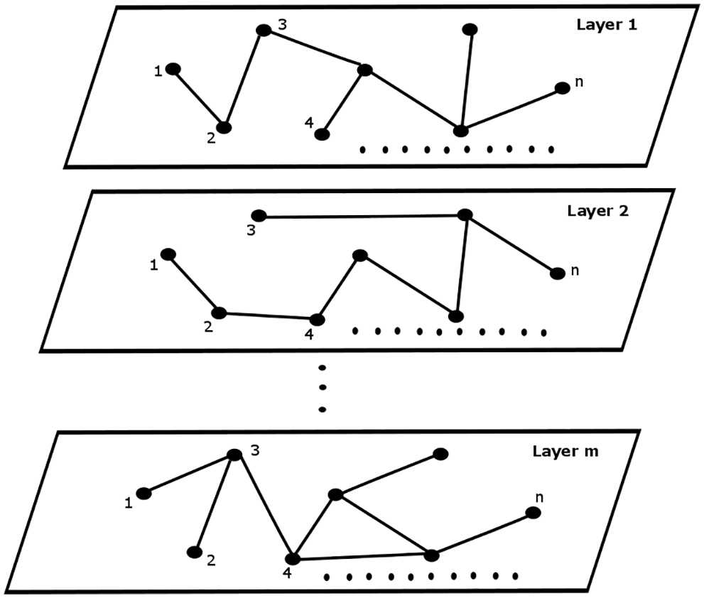
Figure 1: Multiplex network
The approach proposed in [5] uses cosine similarity of nodes present in two different layers and aggregates it in layer level to find similarity between two layers. Their methodology uses a neighborhood-based similarity measure, and it is executed for each and every node. It measures the degree of neighborhood similarity observed by the same node in two different layers. Unlike this proposal, a different notion of layer similarity is used that is not based on neighborhood structure also doesn’t consider all the nodes. Rather the proposed methodology of this paper considers only the common core nodes for evaluation.
Here, a new measure for layer similarity between layers is proposed that is based on number of common cores, average clustering coefficient of common core, and influence capacity of common core. It computes the layer similarity between all possible pair of layers present in the multiplex network M.
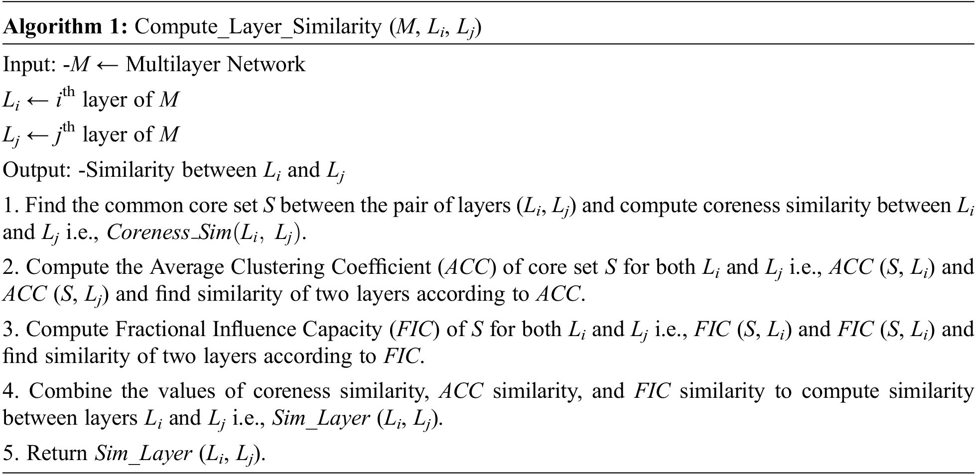
The proposed approach is a combination of three concepts i.e., core, clustering coefficient, and influence/diffusion capacity. The overall approach can be carried out through Algorithm 1, the same is represented via a flowchart in Fig. 2 for clear understanding. Algorithm 1 is computed for all pairs of layers. The steps of the Algorithm 1 are described in the subsequent subsections.
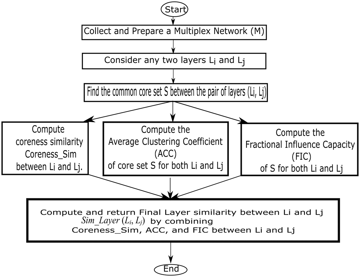
Figure 2: Flow of overall work
5.1 Common Core and Coreness Similarity
The core set of a layer Lk is denoted as Coreset(Lk) i.e., set of nodes present in the core of the layer Lk generated from k-shell decomposition [27] of the layer Lk. The set of common core nodes S between the cores of two layers Li and Lj is the set of nodes present in the core of core-periphery structure of both Li and Lj.
Coreness similarity between two layers Li and Lj is denoted as
where S =
5.2 Average Clustering Coefficient of Common Core
Clustering Coefficient [21] of a node v measures how closely the neighbors of v are connected. It can be computed as:
where k is the actual number of edges between the neighbors of v and
Average Clustering Coefficient (ACC) of the common core set S of layers Li and Lj i.e.,
where CC(v, Li) is the Clustering Coefficient of v in layer Li and | S | is the number of common nodes of layers Li and Lj. The ACC similarity between two layers Li and Lj can be defined as:
where min(ACC(S, Li), ACC(S, Lj)) is the minimum of the average clustering coefficient of S found in Li and Lj. Here, the minimum value of both the components is considered as this degree of similarity must be observed in both the layers. This can be calculated for all pairs of layers.
5.3 Fractional Influence Capacity of Common Core
The influence of a set of nodes is computed by using Independent Cascade Model (ICM) [8] that is similar to Susceptible-Infected (SI) model [17]. At first, all common core nodes (set S) are assumed to be in infected state (seed set) and rest nodes of the layer Li is in susceptible state. The recently infected node can influence its neighbors with a predefined probability p. The infected node gets a single chance to influence/infect its neighbor. The set of total infected nodes is called as cascade set of the common core set S and the cardinality of cascade set is called as cascade capacity (CaC). The average of CaCs over m runs is considered as the Influence Capacity (InC) of the common core in layer Li. Because it obeys Monte-Carlo simulation [28] and produces different cascade capacity in different run. InC for set S in layer Li can be computed as:
where CaCk(S, Li) represents the kth cascade capacity of set S in layer Li.
To make the comparison between the influence capacities of common core set S in two different layers Li and Lj, it is better to compute Fractional Influence Capacity (FIC) that finds the fraction of nodes of the overall nodes in a layer is influenced by the seed set. Because the connection structure of layers in a multiplex network is different. FIC for set S in layer Li can be computed using
where InC(S, Li) represents influence capacity of set S in layer Li, N(Li) is the number of nodes in layer Li. Though the number of nodes present in multiplex network remains same in all layers, the nodes may exhibit different connection patterns in different layers. Hence, the number nodes in the largest connected component of different layers varies. The FIC similarity between two layers Li and Lj can be defined as:
where min(FIC(S, Li), FIC(S, Lj)) i.e., the minimum of the fractional influence capacity of S found in Li and Lj. The minimum value of both the components is considered as it is observed in FICs of both the layers. This can be extended for all pairs of layers.
5.4 Computation of Layer Similarity
The computation of layer similarity between two layers combines three notions of similarity i.e., coreness similarity, average clustering coefficient, and fractional influence capacity. The similarity between two layers Li and Lj i.e., Sim_Layer (Li, Lj) can be computed as:
where
This section presents analysis on the results obtained from the implementation of proposed and existing approaches. The experiments are done by the help of Intel(R) Core(TM) i7-4770 processor (2.40 GHz) with 4GB memory. The programs are written in python and networkx is used as a major tool. Networkx tool is a very powerful tool with enrich set of functionalities that not only provides proper graph visualization but also provides efficient graph programming framework. It is compatible to work with the graph datasets exported from external sources and internal datasets. Models like Erdos-Renyi, Barabasi-Albert, etc [9]. are available for constructing the graph dataset from generative models. In this paper, the graph datasets are collected from external sources and analyzed.
Dataset The experiment includes three real-world multiplex networks: PEDGETT FLORENTINE FAMILIES [29], CS-AARHUS [30], and EU-AIR TRANSPORTATION MULTIPLEX [31].
PEDGETT FLORENTINE FAMILIES is a 2-layer network where two layers are marriage alliances (Layer 1) and business relationships (Layer 2). It contains 16 nodes and 35 edges. Likewise, the CS-AARHUS is a 5 layered network where the layers are Facebook (Layer 1), Leisure (Layer 2), Work (Layer 3), Co-authorship (Layer 4), and Lunch (Layer 5). It contains 61 nodes and 620 edges. The third network EU-AIR TRANSPORTATION MULTIPLEX is a 37 layered network where each layer represents the connection pattern found as per a particular transport service. It has 450 nodes and 3588 edges.
In all the networks the number of nodes remain same in all the layers, whereas the number of edges differ from layer to layer. The total number edges are the sum of number of edges in different layers.
6.1 Illustration with a 2-Layered Network
A complete step-by-step evaluation of the proposed approach is presented for the PEDGETT FLORENTINE FAMILIES dataset. This two-layer multiplex network is shown in Fig. 3. Though the number of nodes is 16, not all the nodes are present in all layers. If a node is not shown in a layer, then it means it is not associated (remain isolated) to any of the other nodes according to the underlying relationship of that layer. The overall process of evaluation is as follows:
1. In Layer 1 (L1) and Layer 2 (L2), the list of core nodes is [9, 2, 7, 3, 5, 4, 11, 15, 16, 13] and [3, 5, 6, 9, 11, 4, 7, 8] respectively. The common set of nodes S between L1 and L2 is [3, 4, 5, 7, 9, 11], and union between the two lists is [2, 3, 4, 5, 6, 7, 8, 9, 11, 13, 15, 16]. The
2. The value of
3. The value of
4. By substituting above values in Eq. (8) the
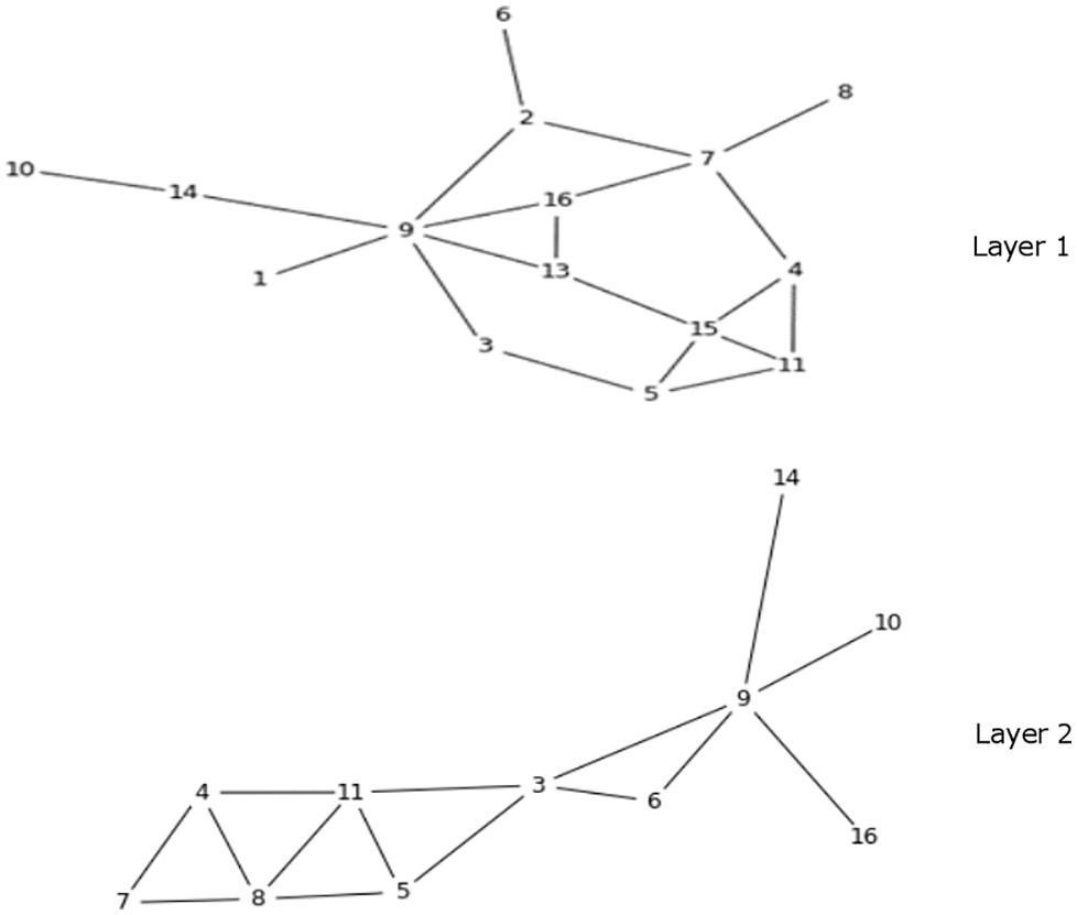
Figure 3: PEDGETT FLORENTINE FAMILIES 2-layer network
Existing approach of layer similarity proposed in [5] is considered that works in two steps: (i) Similarity between the same node k present in two different layer Li and Lj is evaluated using neighborhood-based similarity. (ii) The average of node similarity of all nodes of layer Li and Lj defines layer similarity. The existing method uses cosine similarity to evaluate node similarity. Here, Jaccard coefficient [2] based node similarity is used in place of cosine similarity. The existing approach with Jaccard coefficient follows the given steps.
1. Jaccard coefficient of node k between two different layer Li and Ljcan be computed using
2. Similarity between two layers Li and Lj can be evaluated by using
The correlation between the proposed similarity measure
where
6.4 Evaluation on Network with More Than 2 Layers
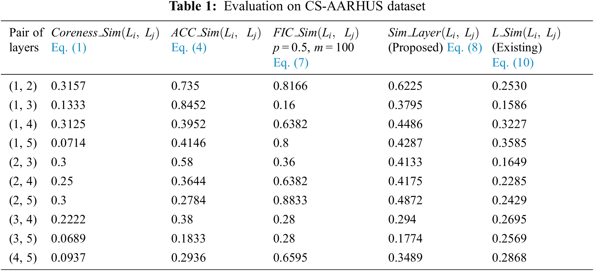
The datasets CS-AARHUS and EU-AIR TRANSPORTATION MULTIPLEX are considered with 5 and 37 layers respectively.
In CS-AARHUS, all 10 pairs (
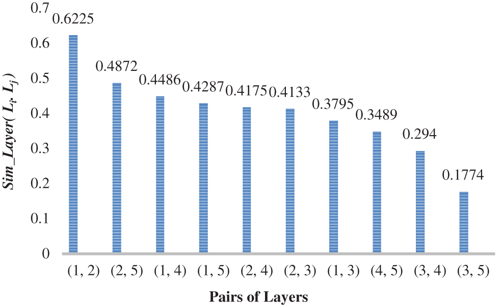
Figure 4: Ranked
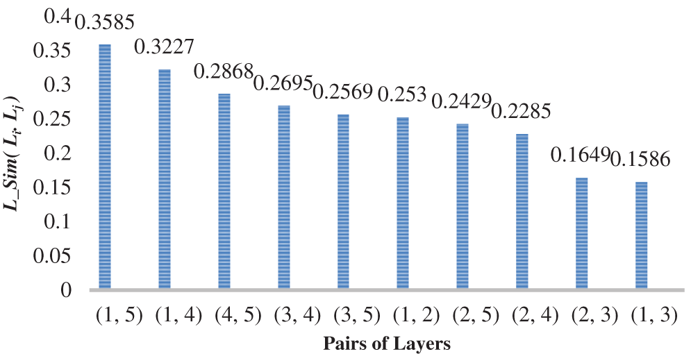
Figure 5: Ranked
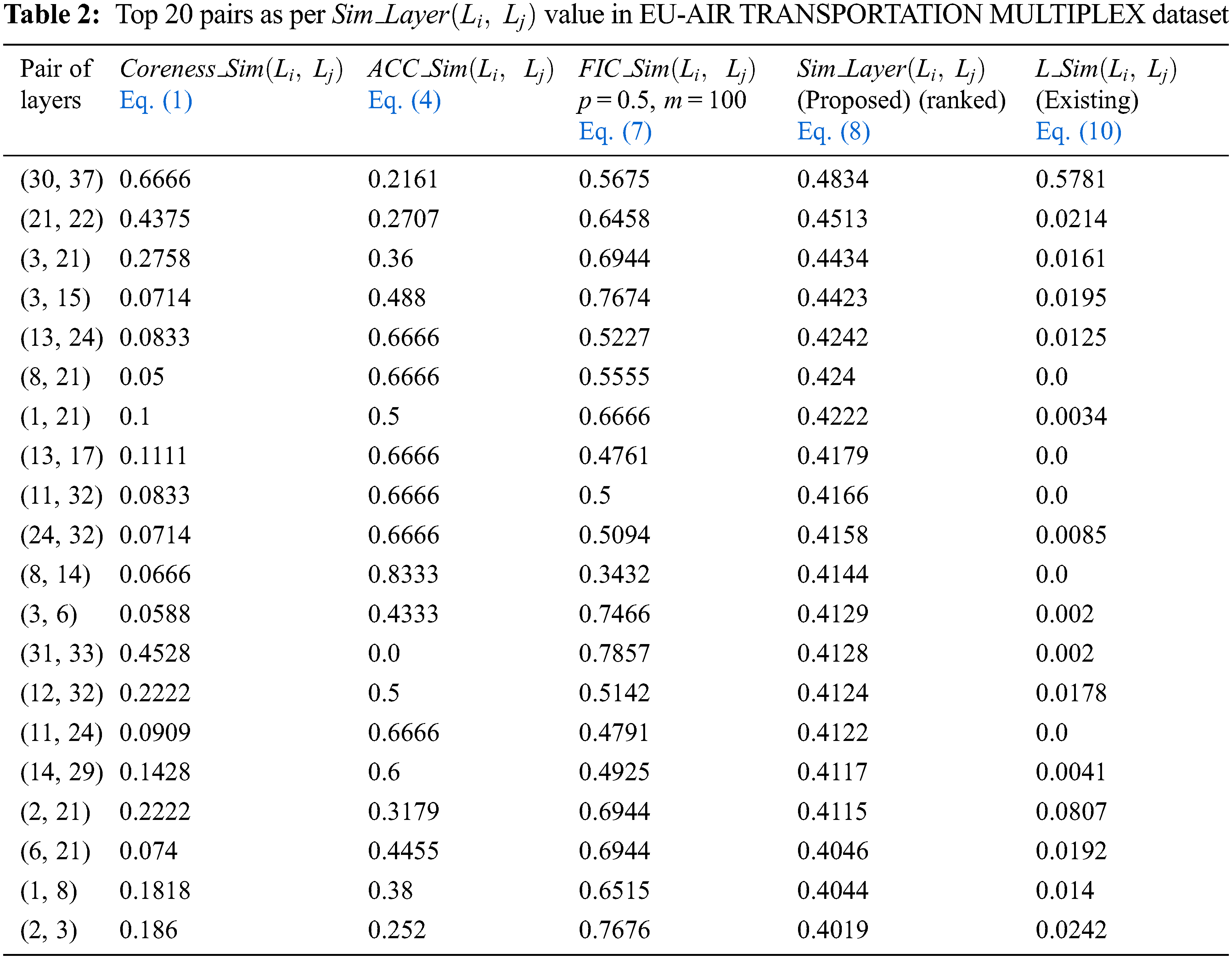
In EU-AIR TRANSPORTATION MULTIPLEX, it is difficult to show the evaluation of layer similarity between all 666 pairs (
This low positive correlation in these two datasets confirms that these two different notions of similarity have their own importance. This proposal emphasizes more on influence and information diffusion aspect whereas the existing method deals with neighborhood structure.
6.4 Degree of Coreness Difference
The evaluation metric, Degree of coreness difference describes the difference in the common core set in two layers as
Fig. 6 shows the number of pairs having degree coreness difference > 0.5 but depicts high degree of layer similarity according to Existing method [5] and Proposed method for both multiplex network datasets under consideration. It is found to be high in case of Existing method [5]. As the proposed method preserves a high degree of coreness similarity, it reports less degree of difference. Again, the % representation of the same is defined using
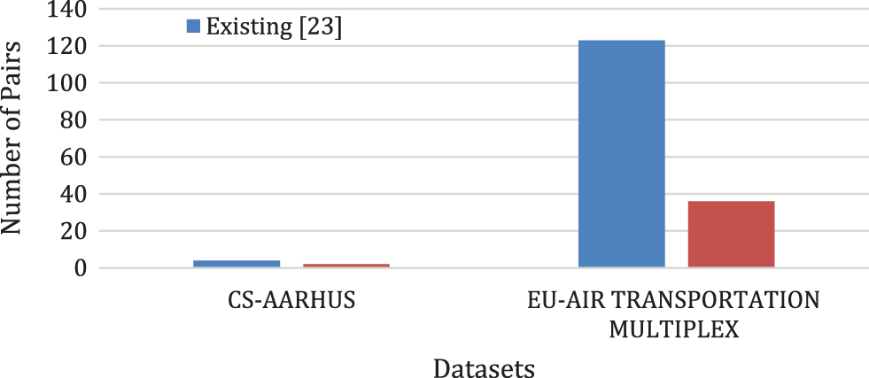
Figure 6: Number of pairs with degree of coreness difference > 0.5
Fig. 7 shows the
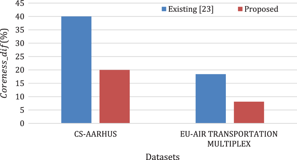
Figure 7: Degree of coreness difference in (%)
6.5 Application of the Layer Similarity
As multiplex network captures multiple relationships among the same set of users, it provides a multi view analysis framework for the same. The computation of layer similarity can be applicable in the task of link prediction. In link prediction [23–26], from different layers of multiplex network, one layer is chosen as target layer. The links of the target layer are categorized into train links and test links. The layer similarity is used to find the similar layers with the target layer and those layers are used for training the model. After training, the accuracy of the model is tested using the test links. Model that passes through testing is used for predicting the missing/upcoming links of the target layer.
This paper proposes a core-based approach to define pairwise layer similarity in a multiplex network. It aggregates the three parameters i.e., number of common cores, average clustering coefficient of common core and fractional influence capacity of common core. This proposal presents a different notion of layer similarity than existing neighborhood-based similarity. The results show a low level of positive correlation between proposed measure
Funding Statement: The authors would like to thank for the support from Taif University Researchers Supporting Project number (TURSP-2020/10), Taif University, Taif, Saudi Arabia.
Conflicts of Interest: The authors declare that they have no conflicts of interest to report regarding the present study.
1. Y. Deng, Z. Jia, G. Deng and Q. Zhang, “Eigenvalue spectrum and synchronizability of multiplex chain networks,” Physica A: Statistical Mechanics and its Applications, vol. 537, no. 122631, pp. 1–20, 2019. [Google Scholar]
2. A. Halu, M. De Domenico, A. Arenas and A. Sharma “The multiplex network of human diseases,” Npj Systems Biology and Applications, vol. 5, no. 15, pp. 1–12, 2019. [Google Scholar]
3. E. A. Horvát and K. A. Zweig, “A fixed degree sequence model for the one-mode projection of multiplex bipartite graphs,” Social Network Analysis and Mining, vol. 3, pp. 1209–1224, 2013. [Google Scholar]
4. S. Jalan and P. Pradhan, “Localization of multilayer networks by optimized single-layer rewiring,” Physical Review E, vol. 97, pp. 042314, 2018. [Google Scholar]
5. R. J. Zhang and F. Y. Ye, “Measuring similarity for clarifying layer difference in multiplex ad hoc duplex information networks,” Journal of Informetrics, vol. 14, no. 1, pp. 100987, 2020. [Google Scholar]
6. S. P. Borgatti and M. G. Everett, “Models of core/periphery structures,” Social Networks, vol. 21, no. 4, pp. 375–395, 2000. [Google Scholar]
7. Y. Gupta, D. Das and S. R. S. Iyengar, “Pseudo-Cores: The terminus of an intelligent viral meme’s trajectory,” In: H. Cherifi, B. Gonçalves, R. Menezes and R. Sinatra (Eds.Complex Networks VII, Studies in Computational Intelligence, vol. 644, pp. 213–226, Cham: Springer, 2016. [Google Scholar]
8. D. Kempe, J. Kleinberg and E. Tardos, “Maximizing the spread of influence through a social network,” Theory of Computing, vol. 11, no. 4, pp. 105–147, 2015. [Google Scholar]
9. D. Mohapatra, A. Panda, D. Gouda and S. S. Sahu, “A combined approach for k-seed selection using modified independent cascade model,” In: A. Das, J. Nayak, B. Naik, S. Pati and D. Pelusi (Eds.Computational Intelligence in Pattern Recognition, Advances in Intelligent Systems and Computing, vol. 999, pp. 775–782, Singapore: Springer, 2020. [Google Scholar]
10. G. Madhu, A. Govardhan, B. S. Srinivas, K. S. Sahoo, N. Z. Jhanjhi et al., “Imperative dynamic routing between capsules network for malaria classification,” CMC-Computers, Materials & Continua, vol. 68, no. 1, pp. 903–919, 2021. [Google Scholar]
11. R. P. Nayak, S. Sethi, S. K. Bhoi, K. S. Sahoo, N. Z. Jhanjhi et al., “TBDDoSA-MD: Trust-based DDoS misbehave detection approach in software-defined vehicular network (SDVN),” CMC-Computers, Materials & Continua, vol. 69, no. 3, pp. 3513–3529, 2021. [Google Scholar]
12. S. K. Mishra, S. Mishra, A. Alsayat, N. Z. Jhanjhi, M. Humayun et al., “Energy-aware task allocation for multi-cloud networks,” IEEE Access, vol. 8, pp. 178825–178834, 2020. [Google Scholar]
13. B. K. Tripathy, K. S. Sahoo, A. K. Luhach, N. Z. Jhanjhi and S. K. Jena, “A virtual execution platform for OpenFlow controller using NFV,” Journal of King Saud University-Computer and Information Sciences, 2020. [Google Scholar]
14. N. Alwash and J. D. Levine, “Network analyses reveal structure in insect social groups,” Current Opinion in Insect Science, vol. 35, pp. 54–59, 2019. [Google Scholar]
15. B. K. Bera, S. Rakshit and D. Ghosh, “Intralayer synchronization in neuronal multiplex network,” The European Physical Journal Special Topics, vol. 228, pp. 2441–2454, 2019. [Google Scholar]
16. J. Iacovacci, Z. Wu and G. Bianconi, “Mesoscopic structures reveal the network between the layers of multiplex data sets,” Physical Review E, vol. 92, pp. 042806, 2015. [Google Scholar]
17. H. Liu, N. Yang, Z. Yang, J. Lin and Y. Zhang, “The impact of firm heterogeneity and awareness in modeling risk propagation on multiplex networks,” Physica A: Statistical Mechanics and its Applications, vol. 539, no. C, 2020. [Google Scholar]
18. R. J. Mondragon, J. Iacovacci J and G. Bianconi, “Multilink communities of multiplex networks,” Plos One, vol. 13, no. (3,pp. e0193821, 2018. [Google Scholar]
19. G. Cencetti and F. Battiston, “Diffusive behavior of multiplex networks,” New Journal of Physics, vol. 21, pp. 035006, 2019. [Google Scholar]
20. S. Gómez, A. Díaz-Guilera, J. Gómez-Gardeñes, C. J. Pérez-Vicente, Y. Moreno et al., “Diffusion dynamics on multiplex networks,” Physical Review Letters, vol. 110, pp. 028701, 2013. [Google Scholar]
21. P. Bródka, A. Chmiel, M. Magnani and G. Ragozini, “Quantifying layer similarity in multiplex networks: A systematic study,” Royal Society Open Science, vol. 5, no. 8, pp. 171747, 2018. [Google Scholar]
22. L. C. Carpi, T. A. Schieber, P. M. Pardalos, G. Marfany, C. Masoller et al., “Assessing diversity in multiplex networks,” Scientific Reports, vol. 9, pp. 4511, 2019. [Google Scholar]
23. S. Bai, Y. Zhang, L. Li, N. Shan and X. Chen, “Effec-tive link prediction in multiplex networks: A topsis method,” Expert Systems with Applications, vol. 177, pp. 114973, 2021. [Google Scholar]
24. S. H. Jafari, A. M. Abdolhosseini-Qomi, M. Asadpour, M. Rahgozar and N. Yazdani, “An information theoretic approach to link prediction in multiplex networks,” Scientific Reports, vol. 11, no. 1, pp. 1–21, 2021. [Google Scholar]
25. F. Karimi, S. Lotfi and H. Izadkhah, “Community-guidedlink prediction in multiplex networks,” Journal of Informetrics, vol. 15, no. 4, pp. 101178, 2021. [Google Scholar]
26. D. Mohapatra, “A hybrid approach for pair-wise layer similarity in a multiplex network,” Social Network Analysis and Mining, vol. 11, no. 88, pp. 1–10, 2021. [Google Scholar]
27. M. Kitsak, L. Gallos, S. Havlin, F. Liljeros, L. Muchnik et al., “Identification of influential spreaders in complex networks,” Nature Physics, vol. 6, pp. 888–893, 2010. [Google Scholar]
28. S. Lv and L. Pan, “Influence maximization in independent cascade model with limited propagation distance,” In: W. Han, Z. Huang, C. Hu, H. Zhang, L. Guo (Eds.Web Technologies and Applications, APWeb 2014, Lecture Notes in Computer Science, vol. 8710, pp. 23–34, Cham: Springer, 2014. [Google Scholar]
29. J. F. Padgett and C. K. Ansell, “Robust action and the rise of the medici, 1400-1434,” American Journal of Sociology, vol. 98, no. 6, pp. 1259–1319, 1993. [Google Scholar]
30. M. Magnani, B. Micenková and L. Rossi, “Combinatorial analysis of multiple networks,” Arxiv, abs/1303.4986, 2013. [Google Scholar]
31. A. Cardillo, J. Gómez-Gardeñes, M. Zanin, M. Romance, D. Papo et al., “Emergence of network features from multiplexity,” Scientific Reports, vol. 3, no. 1344, 2013. [Google Scholar]
32. R. E. Walpole, R. H. Myers, S. L. Myers and K. Ye, “Simple linear regression and correlation”, In: Probability & Statistics for Engineers & Scientists, pp. 413–467, Pearsons Education International, India, 2007. [Google Scholar]
 | This work is licensed under a Creative Commons Attribution 4.0 International License, which permits unrestricted use, distribution, and reproduction in any medium, provided the original work is properly cited. |