DOI:10.32604/iasc.2022.024577
| Intelligent Automation & Soft Computing DOI:10.32604/iasc.2022.024577 | |
| Article |
Steering Behavior-based Multiple RUAV Obstacle Avoidance Control
1Konkuk Aerospace Design-Airworthiness Research Institute (KADA), Konkuk University, Seoul, 05029, Korea
2Department of Computer Science and Engineering, Konkuk University, Seoul, 05029, Korea
3Department of Computer Science and Engineering, Saveetha School of Engineering, Chennai, 602105, India
*Corresponding Author: Dugki Min. Email: dkmin@konkuk.ac.kr
Received: 22 October 2021; Accepted: 15 December 2021
Abstract: In recent years, the applications of rotorcraft-based unmanned aerial vehicles (RUAV) have increased rapidly. In particular, the integration of bio-inspired techniques to enhance intelligence in coordinating multiple Rotorcraft-based Unmanned Aerial Vehicles (RUAVs) has been a focus of recent research and development. Due to the limitation in intelligence, these RUAVs are restricted in flying low altitude with high maneuverability. To make it possible, the RUAVs must have the ability to avoid both static and dynamic obstacles while operating at low altitudes. Therefore, developing a state-of-the-art intelligent control algorithm is necessary to avoid low altitude obstacles and coordinate without collision while executing the desired task. This paper proposes an Artificial Intelligence (AI) based steering behavior algorithm that generates a smooth trajectory by avoiding static and dynamic obstacles. The proposed method uses an obstacle detection algorithm (ODA) and obstacle avoidance algorithm (OAA). An obstacle detection algorithm is used to detect potential threats that fall in the course of flight while reaching the desired target, and obstacle avoidance algorithms use the steering behavior method to generate avoidance trajectory. A PC104 embedded board-based HIL (Hardware in the Loop) simulation environment is developed to validate the proposed algorithm. The proposed algorithm is evaluated by experimenting with a variety of nontrivial scenarios involving static and dynamic obstacles.
Keywords: Steering behaviour method; hardware in the loop; obstacle avoidance control; rotorcraft based unmanned aerial vehicle
In recent years the usage of RUAVs to execute different applications has become increasingly important. The small and flexible design has emerged as the most viable solution for the applications where human free operations are required. Specifically, completing the assigned missions in a coordinated manner attracted much attention nowadays. The usage of these vehicles was not only restricted to military applications. However, it is also employed for civil based applications such as cooperative fire detection [1,2] terrain mapping [3,4] autonomous sensor network assignment for intelligent city applications [5], Air quality measurements [6], smart farming [7,8], search and rescue [9], bridge crack detection [10], smart farming [11], cooperative task execution [12], package delivery [13] and so on. In the applications mentioned earlier, remote-based piloting is an option for largely open airspace. In the case of complex applications like terrain mapping [14], more degree of autonomous behavior is the primary concern, where the RUAVs desire to fly at low altitudes. RUAVs require flying even faster by group coordination, avoiding congested obstacles and terrain-obscuration [15,16].
Due to their limited collision avoidance skills and public security concerns, these applications are still too immature to permit aviation authorities for extensive deployment. Numerous critical technologies should be investigated to ensure that RUAVs can reliably accomplish assigned missions, including collision avoidance and group coordination under aviation legislation. The safety of RUAVs operating in public airspace without human piloting remains a crucial concern. To significantly improve application diversity while minimizing human supervision, the research community should focus more on group collaboration and obstacle avoidance. A possible collision thread is activated if the sensing system verifies that the obstacles are nearing the vehicle trajectory. The obstacle avoidance mechanism pauses the waypoint navigation system’s current trajectory and generates a new trajectory to avoid probable obstructions. Once potential obstacles have been avoided, the vehicle attempt to follow the planned path [17].
The critical operation of a RUAV when flying at a low altitude is to avoid the obstacle in which manual control is not feasible for unpredicted scenarios. In the case of obstacle avoidance situations, the human pilot should have required high skills to formulate the indefinable manipulation. It can be a significant challenge to construct an algorithm that artificially emulates human behavior capabilities to achieve a similar level of litheness and robustness without human operation. To mimic similar maneuverability without human interventions is one of the most challenging tasks. Developing control algorithms that artificially emulate human behavior is another challenge. Based on the environment information, the onboard control system should spontaneously generate a motion command to evade the obstacles while maintaining the desired path and coordinating with peer RUAVs.
In such context, this paper discusses the problem of detection and avoidance of static and dynamic obstacle when the RUAVs fly along with other RUAVs. Therefore, in this work, two control algorithms are addressed they are (a) Obstacle Detection Algorithm (ODA) and (b) Obstacle Avoidance Algorithm (OAA). The contribution of this paper is summarized as follows
• The customized dynamic model for small-scale RUAV is developed and utilized for the simulation of proposed algorithms.
• A two AI-based steering behavior algorithm is proposed. The obstacle detection algorithm detects the possible static and dynamic threads that the falls in the trajectory of the RUAV. The obstacle avoidance algorithm generates a Spatio-temporal trajectory that avoids both dynamic and static obstacles.
• The PC104 embedded hardware-based multiple RUAV HILS testbed is developed to validate the proposed control algorithms.
The rest of the paper is broken out as follows: Section 2 summarizes the current research findings of multi-RUAV obstacle avoidance and group coordination control, followed by Section 3, which describes the RUAV platform guidance law design, Section 4, which presents the proposed multi-RUAV obstacle detection, avoidance, mechanism for executing the desired mission tasks, and in Section 5 the simulation platform for executing the desired mission tasks is briefed. In Section 6, the proposed algorithm is validated with various scenarios. Section 6 discussed the conclusion and future directions.
Intensive research has been carried out in the development of Multiple UAV obstacle avoidances and group coordination control in the past decade. For instance, Yanh Huang et al. presented a Reynolds rule-based collision avoidance strategy for multiple self-organizing RUAV [18]. The method can organize the flights in groups while the collisions are avoided in the desired path. The flocking optimization algorithm is proposed and validated within the simulation environment to ensure a smooth trajectory. In [19], Pavel Petrack used the Reynolds approach for decentralized swarms of RUAV without any communication between the RUAVs or shared absolute localization. Khatib et al. [20] presented an artificial potential fields-based obstacle avoidance algorithm in the real-time scenario. The obstacles are avoided by utilizing the cumulative value of repulsive and attractive forces. The darknet-53 based deep learning approach is prosed by Wang et al. [21] to detect the obstacle and generate the temporal trajectory to avoid it.
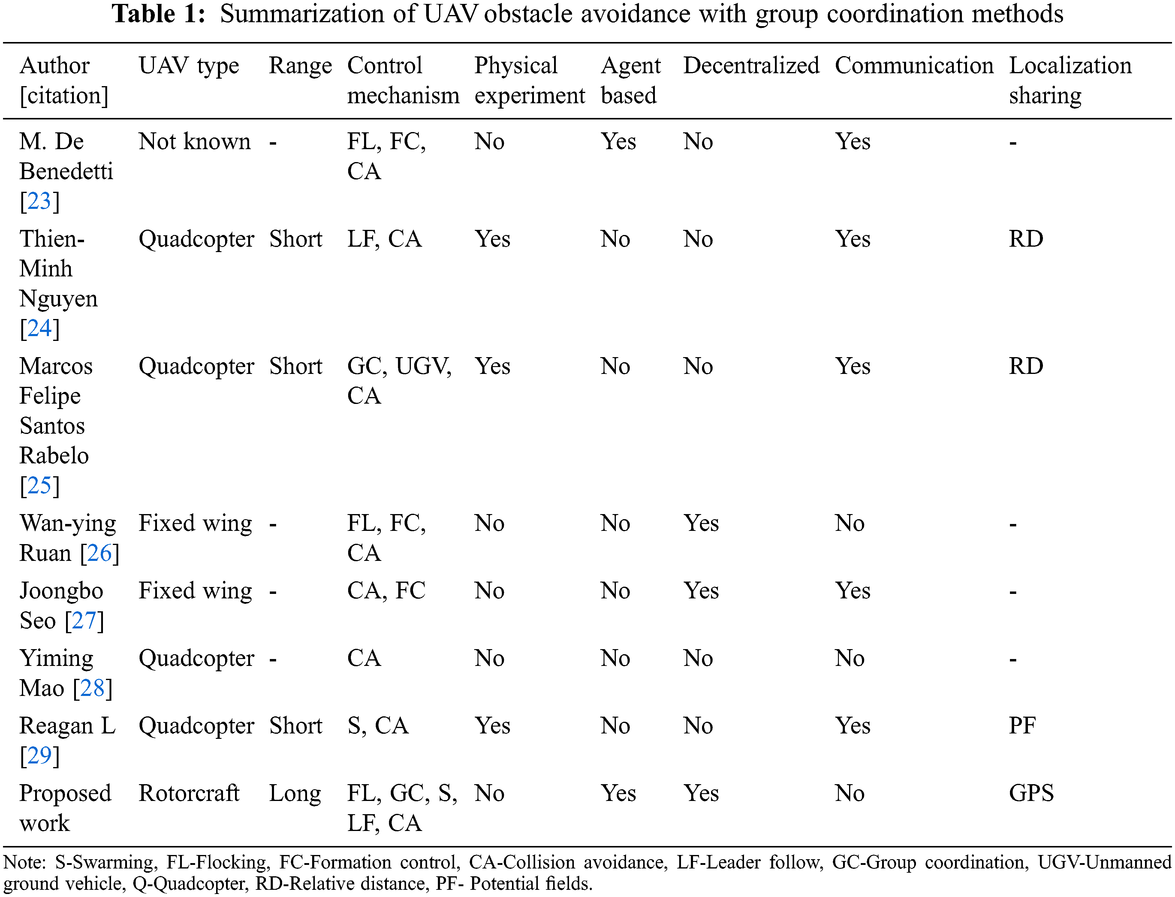
Borenstein et al. [22] demonstrated a real-time obstacle avoidance algorithm using the Virtual Force Field method for mobile robots in which the attractive virtual force (VAF) is applied to the target. In contrast, virtual repulsive force (VRF) is applied to the robot. Tab. 1 consolidates the various algorithms proposed by the research groups across the globe.
The dynamic model of the proposed small-scale RUAV is inspired from [30], which gives the simplified expressions for the motion of a full-scale RUAV. The non-linear equations of motion for the proposed model are presented in this section. Euler-Newton equations based on the law of conservation of linear and angular momentum are derived from Eqs. (1) and (2).
where m denotes the vehicle mass and I represents the inertial tensor.
where
The mathematical expression representing the external forces and moments related to RUAV with respect to its vehicle states and control inputs is derived from the above differential equation. In the case of small-scale RUAV, the forces and moments exerted from the external sources comprise forces produced through the primary and tail rotor, horizontal and vertical fin, aerodynamic forces from the fuselage, and gravitational force. In this experiment, fins are not utilized. Hence, the fuselages and rotors are alone considered.
Main rotor:
The thrust equation of the main rotor can be expressed using Eq. (6)
The main rotor torque can be derived as in Eq. (7)
The main rotors flapping motions can be expressed as in Eq. (8).
Tail rotor:
The expression for thrust equation and velocity component of the tail rotor is given in Eq. (9)
While the tail torque is derived by
Fuselage:
The rotor downwash is deflected through forward as well as side velocity in case of hover and low-speed type of flight. The deflection generated opposes the movement. The expression for fuselage forces of small-scale RUAV is given in Eq. (11).
4 RUAV Obstacle Detection and Avoidance Algorithm
The UAV must forecast and prevent potential threads while maneuvering. In some situations, the projected occurrence of obscurations can be prevented utilizing onboard data such as terrain height and several well-known threads [12]. An anonymous obstacle may occur in real-time circumstances; the algorithm should address these types of obstacles, even if they are small. This section provides an overview of the proposed obstacle identification and avoidance methods developed as a part of point navigation and guidance law.
4.1 Navigation and Guidance Law
The obstacle avoidance system is built using guidance law and point navigation for RUAV reported in [31]. Simulation-based flight control using an autonomous control algorithm is developed in [32]. The proposed guidance law has the advantages of realigning the flight direction using a velocity vector instead of using bank angle value indirectly. The bank angle represents a rotation of the lift force around the velocity vector. The step-by-step procedure of point navigation guidance law is as follows:
Step1: Identify the future position concerning time depending upon the current position (xE,xn) and velocity vector (us(t)). The current position and the velocity of the RUAVs is fetch sensor modules. The location of the RUAVs future north and south (hpfe, hpfn) position is estimated using Eq. (12),
where xE, xn is the north and east location of the RUAV and us(t)E, us(t)N is calculated as
where Vs is the velocity vector, Ws, Wp, Wt are the detection box center points for navigation.
Step2: If the projected future position distance is out of the boundary (dtube < d), then take a new future target point (Wp). The boundary box dtube is assigned twice the size of RUAVs rotor blade.
where Wp is the point located on the line which joins Ws point and Wt point.
In case of Wp value is in out of the specific line, utilize the Wt value as a target point value. d represents the distance between ws and wt.
Fig. 1 illustrates the navigation and control function diagram. The desired side velocity and forward velocity is calculated using Eqs. (16) and (17) [33]
where
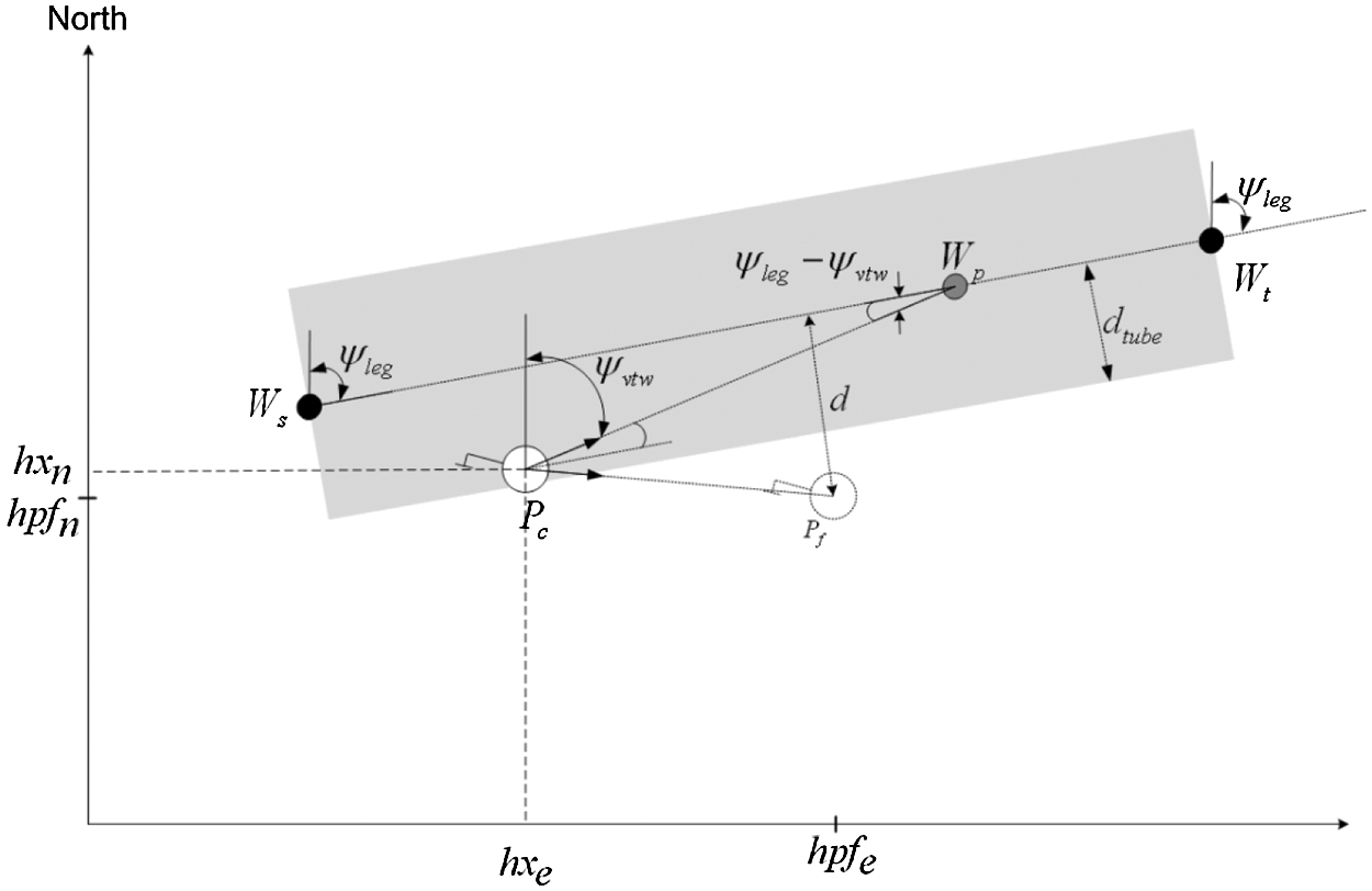
Figure 1: Functional diagram of point navigation for RUAV
The forward speed holding system is built using the control commands as mentioned in Eqs. (18) & (19)
The autopilot systems altitude value, as well as heading hold system, are attained with the help of the command controls from the collective channel, and the rudder channel is expressed by Eqs. (20) and (21)
4.2 Obstacle Detection Algorithm (ODA)
Obstacles are structures that protrude from the flight path and cause RUAVs to collide. The ODA keeps track of the precise geographical coordinates of obstacles likely to cascade along the RUAV path. The navigation component effectively creates the flight path that the RUAV is directed to follow. The flying path directions are preconfigured through the pathway points set up from Ground Control Station (GCS). The starting position is referred to as a base, and the end position is mentioned as a target. The overall pathway points associated from base to endpoint creates a trajectory path. When RUAV follows a predetermined trajectory, ODA must identify any potential threats that are part of the predetermined trajectory. Fig. 2 depicts the conceptual diagram of the obstacle detection process for autonomous RUAV. The following is a step-by-step breakdown of the obstacle identification method:
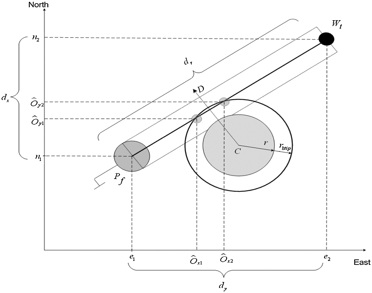
Figure 2: Conceptual diagram of obstacle detection process for RUAV
Step 1: In the initial stage, ODA needs the familiarization of obstacle detection in the scanned area covered by the sensors. If an obstacle is found in the scanned region, it should be tagged with all other probable obstacles to be addressed in the future. According to Reynolds modeling theory, the length of the detected box area is exactly proportional to the vehicle speed. The detection box length (ld) is estimated through Eq. (22) as follows
where ldmin represents the length of the minimum detected box, Gs is the current ground speed, and Sl denotes the scan length.
Step 2: Probable collision detection is computed depending upon the future location of RUAV. The future position Pf can be estimated using Eq. (23)
where Pc and Vc represent the current position and velocity of RUAV.
Step 3: In the computation, any negative value of the barriers with respect to the future position must be ignored. Fig. 3 depicts the omission of negative value falls in the perspective of x-coordinates.
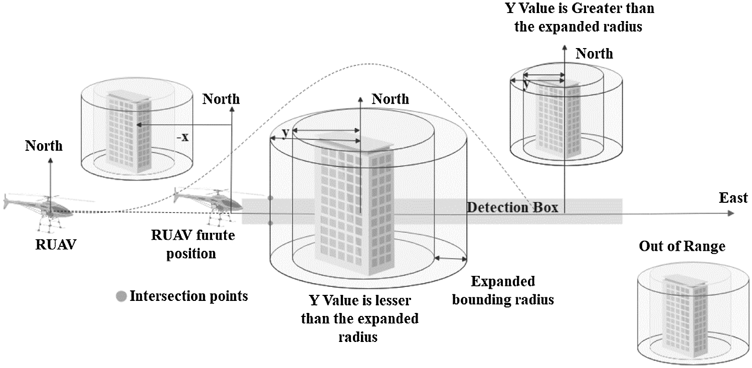
Figure 3: Functional diagram of obstacle detection algorithm for RUAV
Step 4: The proposed algorithm verifies whether the obstacle overlaps on the detected box or not. This condition is achieved by extending the obstacle’s coverage radius to half of the detected box width, also known as the Expanded Bounding Radius (Ebr). The obstacle falling within the bounding region is calculated by the condition “if
Step 5: The remaining obstacles are eliminated, and the intersection test takes into consideration of possible colliding obstacles. The goal of this test is to identify the closest obstacle to which RUAV control must pay attention. As illustrated in Fig. 2, this condition may be obtained by computing the intersection points closure to the RUAV. The obstacle (Pi) is denoted with circle coordinates as (Cx, Cy). The intersection points (
where the function of
Where the other function with respect to the Eqs. (24)–(27) is derived as
Step 6: Line intersection can be achieved with
The center of a circle can be calculated as
Step 7: The closest intersection point is calculated based on line intersection test. The lesser the value of “Pi” is the closest obstacle. Then the obstacle should be considered for avoidance.
Step 8: The nearest obstacle, “Pi” is noted for future examination, while the remaining obstacles are disregarded. Finally, the “Pi” value, which is designated as a low positive number, should be evaluated for the obstacle avoidance algorithm.
4.3 Obstacle Avoidance Algorithm (OAA)
The goal of OAA is to find potential intersection points and compute the angle at which RUAV should avoid them. Two types of forces, lateral and braking force, must be controlled to implement this algorithm [34]. The algorithm is expressed as following steps:
Step 1: Initially, potential intersection points are obtained from ODA. The angle at which the target must be reached is determined and compared to the current angle.
Step 2: The distance between the RUAV’s future position and the obstacle is calculated. The lateral force should be generated to steer the RUAV to avoid the obstacles based on the following condition. “The smaller the distance, the stronger the lateral force.” The lateral force is calculated in Eq. (30)
where ri represents the closest intersecting obstacle radius, Cx, Cy is the x, y coordinates of the center of the circle.
Step 3: The braking force is calculated to slow down the RUAVs when the potential obstacles are cascaded along the desired path. The braking force Bf is related to the distance between the RUAV and the obstacle. Braking force is calculated as follows
where Bw denotes the breaking weight.
The obstacle avoidance and navigation control law run in parallel. When an obstacle is detected, the OAA algorithm generates braking and lateral force. The navigation control seeks to achieve the target by altering the local pathway points after the obstacle has been overcome.
The following expressions are used to calculate the distance between the obstacle and the RUAV.
where de = (hpfn − Cxi), dn = (hpfe − Cyi)
Desired angle (ψd) is calculated through Eq. (34)
The avoidance trajectory and pathway-points as depleted in Fig. 4 are computed using Eqs. (35)–(40).
Figure 4: Conceptual diagram of obstacle avoidance based and waypoint generation
Utilizing hpfn and hpfe which is derived in Section 2
5 Multiple RUAV Experimental Testbed Using HILS
The proposed algorithms are tested in two stages. In the first stage, testing is done for static obstacles, and then the testing is performed for both static and dynamic obstacle conditions. The most effective technique to implement an embedded system under real-time testing conditions is integrating it into a real-plant model. Due to cost constraints, the system is sometimes unable to be validated in a real-time setting. HILS is one of the most feasible techniques to validate the control system’s performance [35]. The proposed system utilized PC104 based xPC target [32]. The real-time multi RUAV HILS system testbed is exemplified in Fig. 5.
Figure 5: (a) Hardware setup of hardware-in-the-loop testbed for multiple RUAV (b) Autonomous RUAVs flying in flight gear environment
The general block diagram of the multiple RUAV HILS for the autonomous system is illustrated in Fig. 6. The proposed multi RUAV HILS system is the extension of our previous research, which is detailed in [31]. The system consists of 4-independent subsystems: flight Gear, autopilot embedded computer with QNX, Ground Control Stations (GCS), and plant model (6 DoF simulator). The flight gear comprises of sensor data emulator and flight visualization computer. Simulation library in bridging applications is used to link with FlightGear and then connect to PC104 board, emulating outputs and inputs acquired from the RUAV model. Output from the RS232 of the Flight control computer (FCC) is in packed binary format which is similar to the packet produced by the dynamic model and FlightGear and also receives output commands from GCS. The plan model utilise the model proposed in Section 3. This setup mimics the real-time testbed of the rest of the system components. FlightGear transfers the raw data to the FCC. The data communication between the modules are multiplexed and in international system of units [36]. HILS bridging module converts the data before passing them to the PC104 board. Similarly, the raw data format of the HILS Bridge transmits the normalized locations of RUAV dynamic plant models, and the control surface position acquired from the PC104 board is in this format [37].
Figure 6: Hardware setup of HIL simulation for multi RUAV system
6 Experimental Results and Analysis
The performance of the proposed algorithms is validated with the proposed multiple RUAV HILS platform in two phases. In the first phase, a single RUAV is used to check the single and multiple static obstacles. On the other hand, multiple RUAV test beds are utilized to test static and dynamic obstacles in the second phase. The accomplished results based on the simulation setup are presented in this section.
6.1 Test Results of Static Obstacles
The RUAV in the first phase flies in an anticlockwise direction to reach each pathway point and then return to its original starting position. The altitude consider for this simulation is 10 meters. Different sizes of obstacles are purposely placed in the center of the flying zone in this simulation study to validate the proposed algorithm. The ODA should recognize the obstacles, and OAA should compute the trajectory in order to avoid them and reach the desired destination. Fig. 7a shows the RUAV avoided the single static obstacle placed at (0, 35) coordinates with the size of 2.5 meter intelligently.
Figure 7: (a) OAA with single static thread, (b) OAA with multiple static threads
In the second experiment, the RUAV needs to fly in an anticlockwise manner to reach the designated pathway points and return to the target location. The obstacles of various sizes are purposely placed in the center of the flight trajectory. The ODA and OAA should identify the precise size of the obstacles and calculate a trajectory to reach the intended target location while avoiding the obstacles as efficiently as possible. In this simulation study, three different types of obstacles are placed to validate the performance of the proposed algorithm. The coordinates of the obstacles are (30, 10), (0, −30), and (0, 40), with obstacle sizes of 4, 3.5, and 6 meters respectively. The simulation results reveal that the proposed algorithm smoothly avoided the obstacles of various sizes, as shown in Fig. 7b. The various types of trajectory generated at the time of course of flight are illustrated in Fig. 8.

Figure 8: Trajectory generated during the course of flight for multiple static obstacle (a) RUAV altitude (b) RUAV yaw rate (c) RUAV pitch angle (d) RUAV roll angle
6.2 Test Results for Multiple Static and Dynamic Obstacles
The proposed algorithm is then evaluated for both static and dynamic obstacles in the second phase. In this phase, two RUAVs are utilized; RUAV1 flies clockwise and RUAV2 flies in an anticlockwise direction. Multiple static obstacles with different sizes are placed in the RUAV’s desired path. From Fig. 9 it is observed that the effectiveness of the proposed algorithm. The algorithm smoothly avoids both the static and dynamic obstacles while in the course to reach the target. The various types of trajectory generated at the time of course of flight are illustrated in Fig. 10.
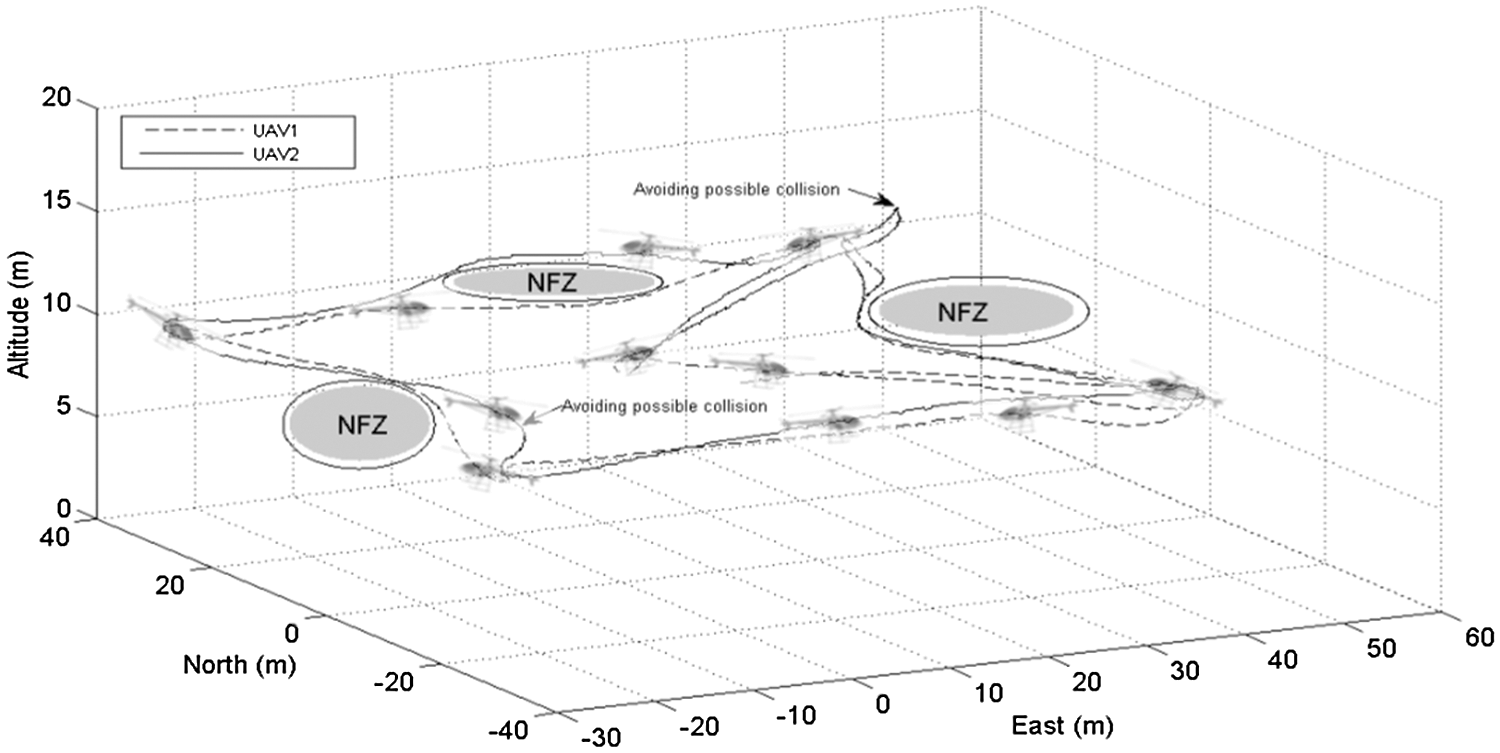
Figure 9: OAA with multiple static and dynamic threads
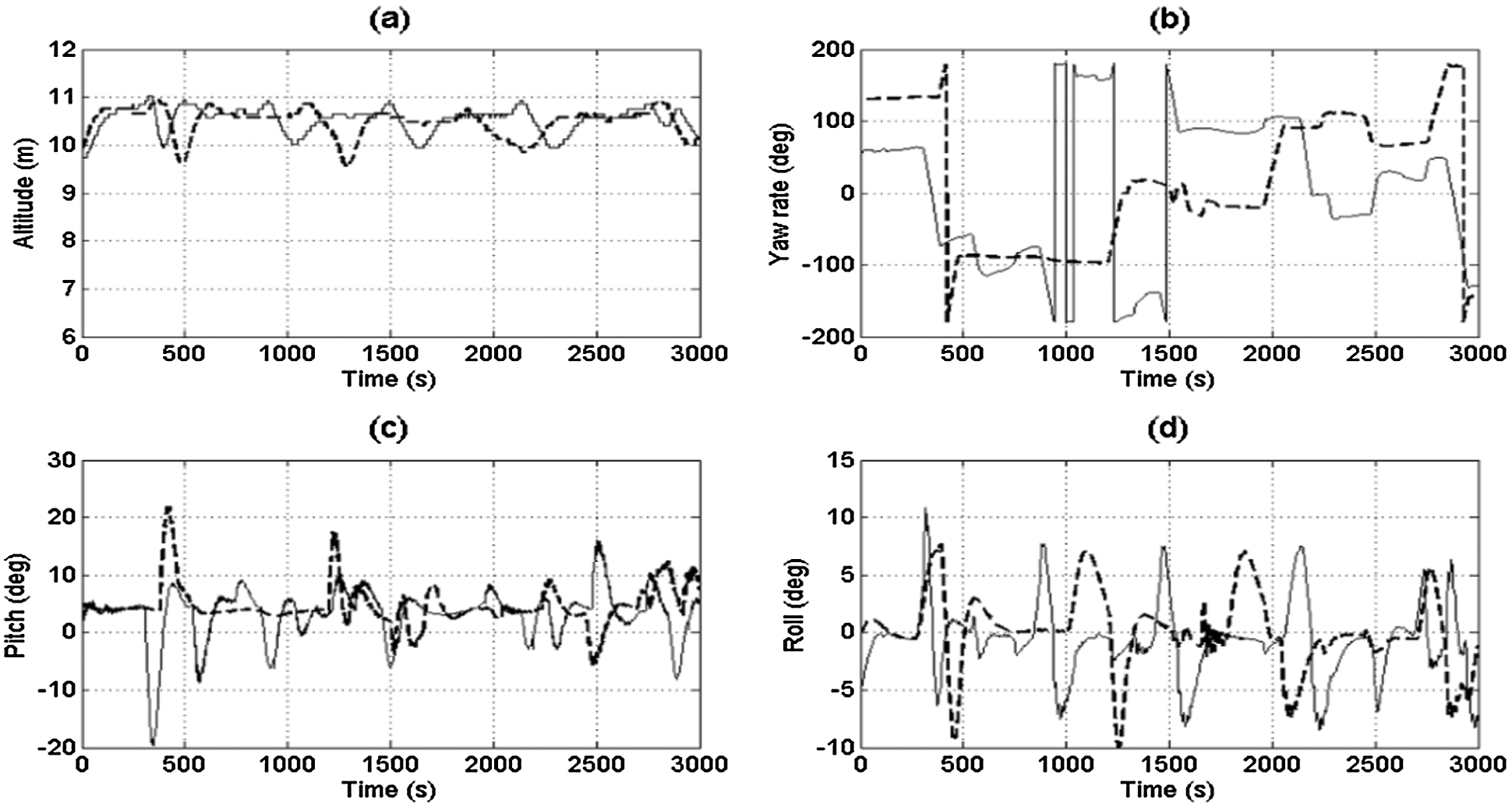
Figure 10: Trajectory generated during the course of flight for multiple static and dynamic obstacle (a) RUAV altitude (b) RUAV yaw rate (c) RUAV pitch angle (d) RUAV roll angle
In order for RUAVs to function properly, they must first identify and avoid obstacles in their flight path, as well as prevent colliding with each other. Robust unmanned aerial vehicles (RUAVs) require a high degree of flexibility to react to changing environments along their flight route. A steering behavior algorithm based on artificial intelligence is used in this work to address the issues and obstacles encountered by the RUAV when responding to both static and dynamic obstructions along its flight trajectory path. For the purposes of this investigation, both obstacles have been intentionally placed in the flight route to test if the proposed algorithm can recognize and avoid them while using the bare minimum of computational resources during the flight. The proposed technique is implemented on a PC104 integrated board running the QNX real-time operating system, and the results are demonstrated and proven in the HILS simulation environment.
Funding Statement: This research was supported by the Basic Science Research Program through the National Research Foundation of Korea (NRF) funded by the Ministry of Education (No. 2020R1A6A1A03046811). This work was supported by the National Foundation of Korea (NRF) Grant funded by the Korea government (Ministry of Science and ICT (MIST)) (No. 2021R1A2C209494311)
Conflicts of Interest: The authors declare that they have no conflicts of interest to report regarding the present study.
1. L. Merino and A. Ollero, “Computer vision techniques for fire monitoring using aerial images,” in IECON Proc. (Industrial Electronics Conf.), IEEE, Seville, Spain, pp. 2214–2218, 2002. [Google Scholar]
2. S. Sudhakar, V. Vijayakumar, C. Sathiya Kumar, V. Priya, L. Ravi et al., “Unmanned aerial vehicle (UAV) based forest fire detection and monitoring for reducing false alarms in forest-fires,” Computer Communications, vol. 149, pp. 1–16, 2020. [Google Scholar]
3. N. M. Zahari, M. A. A. Karim, F. Nurhikmah, N. A. Aziz, M. H. Zawawi et al., “Review of unmanned aerial vehicle photogrammetry for aerial mapping applications,” in Proc. of the Int. Conf. on Civil, Offshore and Environmental Engineering, pp. 669–676. Springer, Singapore, 2021. [Google Scholar]
4. L. S. Santana, G. A. E. Silva Ferraz, D. Bedin Marin, B. Dienevam Souza Barbosa, L. Mendes Dos Santos et al., “Influence of flight altitude and control points in the georeferencing of images obtained by unmanned aerial vehicle,” European Journal of Remote Sensing, vol. 54, no. 1, pp. 59–71, 2021. [Google Scholar]
5. H. Teng, M. Dong, Y. Liu, W. Tian and X. Liu, “A Low-cost physical location discovery scheme for large-scale internet of things in smart city through joint use of vehicles and UAVs,” Future Generation Computer Systems, vol. 118, pp. 310–326, 2021. [Google Scholar]
6. T. F. Villa, F. Gonzalez, B. Miljievic, Z. D. Ristovski and L. Morawska, “An overview of small unmanned aerial vehicles for air quality measurements: Present applications and future prospectives,” Sensors (Switzerland), vol. 16, no. 7, pp. 1072, 2016. [Google Scholar]
7. P. K. R. Maddikunta, S. Hakak, M. Alazab, S. Bhattacharya, T. R. Gadekallu et al., “Unmanned aerial vehicles in smart agriculture: Applications, requirements, and challenges,” IEEE Sensors Journal, vol. 21, no. 16, pp. 17608–17619, 2021. [Google Scholar]
8. A. D. Boursianis, M. S. Papadopoulou, P. Diamantoulakis, A. L. Tsakalidi, P. Barouchas et al., “Internet of things (IoT) and agricultural unmanned aerial vehicles (UAVs) in smart farming: A comprehensive review,” Internet of Things, pp. 100187, 2020. [Google Scholar]
9. M. A. Goodrich, B. S. Morse, D. Gerhardt, J. L. cooper, M. Quigley et al., “Supporting wilderness search and rescue using a camera-equipped mini UAV,” Journal of Field Robotics, vol. 25, no. 1–2, pp. 89–110, 2008. [Google Scholar]
10. Y. Z. Ayele, M. Aliyari, D. Griffiths and E. L. Droguett, “Automatic crack segmentation for uav-assisted bridge inspection,” Energies, vol. 13, no. 23, pp. 6250, 2020. [Google Scholar]
11. P. Mohan and R. Thangavel, “Resource selection in grid environment based on trust evaluation using feedback and performance,” American Journal of Applied Sciences, vol. 10, no. 8, pp. 924–930, 2013. [Google Scholar]
12. V. K. Kaliappan, H. Yong, D. Min and A. Budiyono, “Behavior-based decentralized approach for cooperative control of a multiple small scale unmanned helicopter,” in IEEE Int. Conf. on Intelligent Systems Design and Applications, ISDA, Cordoba, Spain, pp. 196–201, 2011. [Google Scholar]
13. N. Mathew, S. L. Smith and S. L. Waslander, “Planning paths for package delivery in heterogeneous multirobot teams,” IEEE Transactions on Automation Science and Engineering, vol. 12, no. 4, pp. 1298–1308, 2015. [Google Scholar]
14. D. Wierzbicki and M. Nienaltowski, “Accuracy analysis of a 3D model of excavation, created from images acquired with an action camera from low altitudes,” ISPRS International Journal of Geo-Information, vol. 8, no. 2, pp. 83, 2019. [Google Scholar]
15. S. Scherer, S. Singh, L. Chamberlain and S. Saripalli, “Flying fast and low among obstacles,” in Proc.-IEEE Int. Conf. on Robotics and Automation, Rome, Italy, pp. 2023–2029, 2007. [Google Scholar]
16. A. Stentz, “Optimal and efficient path planning for partially-known environments,” in: Proc.-IEEE Int. Conf. on Robotics and Automationm, Boston, MA, pp. 203–220, 1994. [Google Scholar]
17. Z. Liu and A. G. Foina, “An autonomous quadrotor avoiding a helicopter in low-altitude flights,” IEEE Aerospace and Electronic Systems Magazine, vol. 31, no. 9, pp. 30–39, 2016. [Google Scholar]
18. Y. Huang, J. Tang and S. Lao, “Collision avoidance method for self-organizing unmanned aerial vehicle flights,” IEEE Access, vol. 7, pp. 85536–85547, 2019. [Google Scholar]
19. P. Petráček, V. Walter, T. Báča and M. Saska, “Bio-inspired compact swarms of unmanned aerial vehicles without communication and external localization,” Bioinspiration and Biomimetics, vol. 16, no. 2, pp. 026009, 2021. [Google Scholar]
20. O. Khatib, “Real-time obstacle avoidance for manipulators and mobile robots,” International Journal of Robotics Research, vol. 5, no. 1, pp. 396–404, 1986. [Google Scholar]
21. D. Wang, W. Li, X. Liu, N. Li and C. Zhang, “UAV environmental perception and autonomous obstacle avoidance: A deep learning and depth camera combined solution,” Computers and Electronics in Agriculture, vol. 175, pp. 105523, 2020. [Google Scholar]
22. J. Borenstein and Y. Koren, “Real-time obstacle avoidance for fast mobile robots in cluttered environments,” in IEEE Int. Conf. on Robotics and Automation, Cincinnati, OH, USA, pp. 572–577, 1990. [Google Scholar]
23. M. Sundaram, S. Satpathy and S. Das, “An efficient technique for cloud storage using secured de-duplication algorithm,” Journal of Intelligent & Fuzzy Systems, vol. 42, no. 2, pp. 2969–2980, 2021. [Google Scholar]
24. T. M. Nguyen, Z. Qiu, T. H. Nguyen, M. Cao and L. Xie, “Distance-based cooperative relative localization for leader-following control of MAVs,” IEEE Robotics and Automation Letters, vol. 4, no. 4, pp. 3641–3648, 2019. [Google Scholar]
25. M. F. S. Rabelo, A. S. Brandao and M. Sarcinelli-Filho, “Landing a uav on static or moving platforms using a formation controller,” IEEE Systems Journal, vol. 15, no. 1, pp. 37–45, 2021. [Google Scholar]
26. W. Ying Ruan and H. Bin Duan, “Multi-UAV obstacle avoidance control via multi-objective social learning pigeon-inspired optimization,” Frontiers of Information Technology and Electronic Engineering, vol. 21, no. 5, pp. 740–748, 2020. [Google Scholar]
27. J. Seo, Y. Kim, S. Kim and A. Tsourdos, “Collision avoidance strategies for unmanned aerial vehicles in formation flight,” IEEE Transactions on Aerospace and Electronic Systems, vol. 53, no. 6, pp. 2718–2734, 2017. [Google Scholar]
28. Y. Mao, M. Chen, X. Wei and B. Chen, “Obstacle recognition and avoidance for UAVs under resource-constrained environments,” IEEE Access, vol. 8, pp. 169408–169422, 2020. [Google Scholar]
29. R. L. Galvez, G. E. U. Faelden, J. M. Maningo, R. C. S. Nakano, E. P. Dadios et al., “Obstacle avoidance algorithm for swarm of quadrotor unmanned aerial vehicle using artificial potential fields,” in IEEE Region 10 Annual Int. Conf., Proc./TENCON, Penang, Malaysia, pp. 2307–2312, 2017. [Google Scholar]
30. V. Gavrilets, “Autonomous Aerobatic Maneuvering of Miniature Helicopters,” PhD diss., Massachusetts Institute of Technology, 2003. [Google Scholar]
31. V. K. Kaliappan, H. Yong, M. Dugki, E. Choi and A. Budiyono, “Reconfigurable intelligent control architecture of a small-scale unmanned helicopter,” Journal of Aerospace Engineering, vol. 27, no. 4, pp. 04014001, 2014. [Google Scholar]
32. B. Karthikeyan, T. Sasikala and S. B. Priya, “Key exchange techniques based on secured energy efficiency in mobile cloud computing,” Applied Mathematics & Information Sciences, vol. 13, no. 6, pp. 1039–1045, 2019. [Google Scholar]
33. T. Ravichandran, “An efficient resource selection and binding model for job scheduling in grid,” European Journal of Scientific Research, vol. 81, no. 4, pp. 450–458, 2012. [Google Scholar]
34. C. W. Reynolds, “Steering behaviors for autonomous characters,” Game Developers Conference, vol. 41, pp. 763–782, 1999. [Google Scholar]
35. V. K. Kaliappan, A. Budiyono, D. Min, K. Muljowidodo and S. A. Nugroho, “Hardware-in-the-loop simulation platform for the design, testing and validation of autonomous control system for unmanned underwater vehicle,” Indian Journal of Marine Sciences, vol. 41, no. 6, pp. 575–5810, 2012. [Google Scholar]
36. V. D. Ambeth Kumar, S. Malathi, A. Kumar and K. C. Veluvolu, “Active volume control in smart phones based on user activity and ambient noise,” Sensors, vol. 20, no. 15, pp. 4117, 2020. [Google Scholar]
37. P. Subbulakshmi, M. Prakash and V. Ramalakshmi, “Honest auction based spectrum assignment and exploiting spectrum sensing data falsification attack using stochastic game theory in wireless cognitive radio network,” Wireless Personal Communications, vol. 102, no. 2, pp. 799–816, 2018. [Google Scholar]
 | This work is licensed under a Creative Commons Attribution 4.0 International License, which permits unrestricted use, distribution, and reproduction in any medium, provided the original work is properly cited. |