DOI:10.32604/iasc.2022.023455
| Intelligent Automation & Soft Computing DOI:10.32604/iasc.2022.023455 | |
| Article |
Crack Detection in Composite Materials Using McrowDNN
1Department of CSE, Coimbatore Institute of Technology, Coimbatore, India
2Department of ECE, Coimbatore Institute of Technology, Coimbatore, India
*Corresponding Author: R. Saveeth. Email: saveeth.r@cit.edu.in
Received: 09 September 2021; Accepted: 16 December 2021
Abstract: In the aerospace industry, composite materials are becoming more common. The presence of a crack in an aircraft makes it weaker and more dangerous, and it can lead to complete fracture and catastrophic failure. To predict the position and depth of a crack, various methods have been developed. For aircraft repair, crack diagnosis is extremely important. Even then, due to uncertainties arising from sources such as environmental conditions, packing, and intrinsic material property changes, accurate diagnosis in real engineering applications remains a challenge. Deep learning (DL) approaches have demonstrated powerful recognition potential in a variety of fields in recent years. In comparison to conventional artificial neural networks, which have the ability to perform better crack recognition, the Deep Neural Network (DNN) is able to improve the pattern features and achieve better pattern recognition. In this study, DNN-based crack detection in composite material method called Modified Crow Deep Neural Network (McrowDNN) is proposed. The preparation of a Mcrow-based DNN is carried out here in order to choose the most appropriate weights and prejudices. The results show that the proposed method outperforms current methods like Artificial Neural Network (ANN), Recurrent Neural Network (RNN) and Crow Search Algorithm (CSA).
Keywords: Composite materials; aerospace industry; deep learning; convolutional neural network
Since the last few decades, composite materials have been used in a variety of machining and manufacturing processes. Composite materials are so named because they are made up of two or more materials, one of which is a continuous matrix process in which one of the materials, the fiber, is dispersed. The two materials combine to have material properties that are distinct from those of the original elements on their own [1]. Despite the fact that most aeroplanes today are made of aluminium, composite materials such as carbon fibers, glass fibers, and Kevlar, to name a few, are commonly used in the aircraft industry. For example, glass fibers were first used in aircraft by Boeing in the 1950s. Also, Boeing 787 Dreamliner was the first commercial aircraft to be made from 50% composite materials, mainly carbon fiber composites [2].
Crack control is a key concern for safety-critical structures such as aircraft, wind turbines, bridges and nuclear power plants [3]. The issue of ensuring accurate and effective safety controls has received a great deal of attention in recent years in aeronautical contexts, maintenance operations, in particular those carried out on in-service aircraft, must be reliable but must also be carried out at a low cost in order to meet out regular timetables. In particular, techniques of non-destructive testing and evaluation (NDT&E) are important for the early detection of damage to the structure’s high stress and tired area. The study of the transfer of various signals such as ultrasonic, acoustic absorption, heat graphical, laser ultrasound, x-radiographic, eddy current, scanning and low frequency methods are used in some of these NDT&E techniques [4].
Deep learning (DL) has demonstrated its strong acceptance in recent years. As one of the essential approaches in DL, the convolution neural network (CNN), which has the capacity to amplify recognition-related feature representation layer by layer, can be extracted with convolution and consolidation. Components including reactor-metallic surfaces [5], bearing components, planetary gearbox [6] and etc. have been tried in CNN in crack diagnostics. However, there is no literature on fatigue crack diagnosis of DNN aircraft structures. In this paper, an early diagnosis of crack detection based on McrowDNN is proposed in the composite material process. The main contribution of the work is as follows:
• Initially the real time crack and non-crack images of aircraft composite materials are collected and given as input to the proposed McrowDNN method.
• In proposed method, initially the input images are pre-processed by image resizing and sobel edge detector
• Then, Hough transformative properties are extracted, and the result of fatigue cracks is predicted further, using McrowDNN’s crack and non-crack results and real-time crack and non-crack images verification were performed.
• The results show that this method can identify the existence of crack in aircraft structure and is promising for further research.
The rest of the paper is structured as follows: related works on crack detection in plane are discussed in Section 2. The proposed McrowDNN is explained in Section 3 and the experimental results with discussion are given in Section 4. Finally, in Section 5 the conclusion and future work is specified.
Structural health monitoring (SHM) has in recent years been directed toward a big data issue which must be addressed by deep learning. The [7] model-aided deep education approaches to the detection and localization of structural damage combined with ultrasonic waves were given. However, the subject of our future research may be large-scale applications involving complex geometries and multiple harm scenarios. In [8] a neural system model was created to predict the mechanical characteristics (modulus, strength and tightening) of 2D composites. The model exhibits extremely promising capabilities. The ability to use CNN models in the study of structures and materials is seen. CNN models have the ability to speed up existing techniques of optimization and to revolutionize the design of structures and materials.
In [9] a deep-learning method was presented which allows damage features to be extracted from modern forms without any manual feature or previous knowledge. Using the CNN algorithm to develop new network architecture to satisfy the different harm scenario requirements. Also this method achieves a predictive effect, but the results are based on the numerical and laboratory simulations data. This will concentrate on real systems and explore dynamic scenarios as the next phase of this study. In [10], they provided an example of how to integrate field expertise in the creation of profound learning algorithms from aviation engineering. The use of fatigue testing data from aerospace-grade aluminum specimen to create a deep convolutional neural network that classifies crack length by crack propagation curve, obtained from the fatigue test, demonstrates the suitability of our method.
In [11] a framework to classify defects in composite materials by incorporating an in-depth learning technique thermography tests. A data set was compiled from literature and used to train the systems for identifying the defects in thermographic images. The data set consists of composites with defects in thermography. In [12] a CNN approach to the classification and prediction of different forms of flat and thick delamination in smart composite laminates using low-frequency structural vibration outputs was produced. But the majority of these procedures are non-automatic and subjectively determined by operators for diagnostic results.
In [13] the efficiency of various NDT methods for aircrafts composed of different composites typically damaged by aircrafts was studied. Three structures have been considered: glass fiber-reinforced plastic (GFRP) core, the Multi-layered aluminum alloy glass fiber-reinforced plastic (GFRP-Al) platform and two layers of Aluminum alloy on the top and bottom, with a carbon fiber-reinforced plastic (CFRP) structure extracted from an aircraft’s weakened Vertical Stabilizer. In [14], a model for deep transfer learning was used to properly remove defects from aerospace composite material (ACM) with limited sample size for use in X-ray pictures. An automated detection method for X-ray images of ACM has been investigated in this model. Each method has its own advantages and disadvantages, but regional crack detection is much sought after to localize cracked areas especially for automatic inspection on concrete surfaces.
In [15] the Residual Neural Network has been used to automatically identify surface cracks on the road and on the pavements. The large variance in surface texture and the varying light levels render it difficult to detect defects automatically within public and private infrastructures. The device is designed using an ANN feed-forward-architecture feature pyramid heart. In [16] a concrete pavement crack detection model was implemented, with the use of RNN to identify the original images and extract crack features for detection. However, one disadvantage of existing methods is that they are built to recognize cracking coarsely, cracks assuming to be equal to that of the patches. Current methods use Convolutional Neural Network (CNNs) [17,18] In order to work out, assume the whole image would be classified as a crack of just 16 × 16 in an image format 256 × 256. Patches can’t be identified by these coarse methods if cracks are detected at a finer level, such as 16 × 16. The latest methods should also be recycled and costly because of numerous scans needed to identify cracks at the scan window’s edges. There is also a need to retrain the current methods which are costlier in computational terms due to many scans necessary for detecting cracks on the window edges. Thus the new method of crack detection based on CNN-scratch is designed to solve this problem in the proposed work. Both datasets are made up of Carbon Fiber Reinforced Epolam 2063 Resin and dataset 1 shown in Fig. 1 are captured by Evolution VF (1392 × 1040) camera and dataset 2 shown in Fig. 2 were captured by Scanning Electron Microscope (SEM) machine respectively.
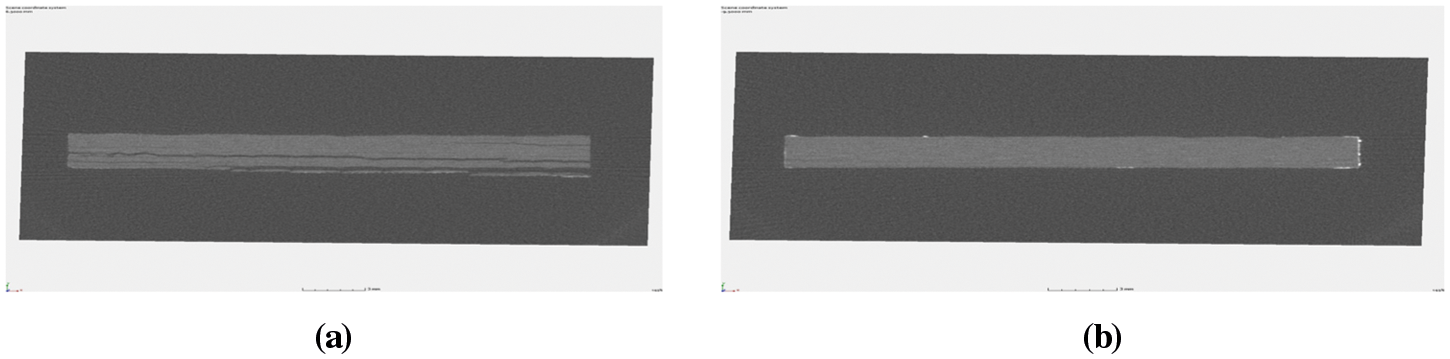
Figure 1: Data set 1: Composite material image (a) Cracks (b) Non-crack image
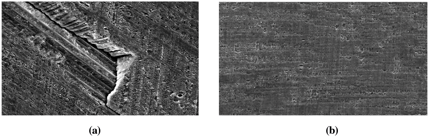
Figure 2: Data set 2: Composite material image (a) Cracks (b) Non-crack image
The Proposed method consists of three modules, (i) acquiring database images of crack in aircraft composite materials, (ii) training the database images using McrowDNN, and (iii) testing that has been done using MATLAB. The architecture diagram of proposed methodology is illustrated in Fig. 3.
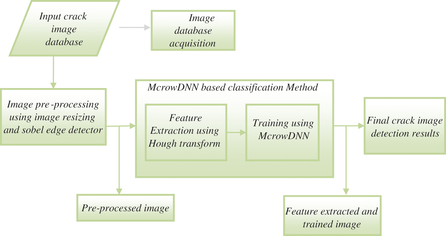
Figure 3: Proposed McrowDNN based crack detection architecture
The raw images have noise interference effect, so it cannot be processed directly. Before examination it is important to pre-process it. The data set of the image is given and the preprocessing of the image is carried out. The image preprocessing involves the re-dimensioning of the image. The pictures are taken with high resolution device, so image size is extremely high. The further processing may take longer, due to the large size of the image, to resize all images to 200 × 200 PX.
3.2 Edge Detection Using a Sobel Operator
Edge Detection is a mathematical procedure that detects image luminosity changes. In a series of curved segments called edges, the points in which the difference in image brightness is abrupt are arranged. These borders are used to look at shifts in environmental characteristics. For greater distinction between borders and surrounding portions of the image, the articulated edges are dilated after the edge detection process. For edge detection in this work, sobel operator [18] is used. It is based on calculations which approximate an image intensity gradient value. The famous Sobel edge-detection operator, which again consists of two masks to define the edge in vector form, doubles the weight at the central pixels of both Prewitt templates. Up until the advent of theoretical border detection methods The Sobel operator was the most common edge detection operator. It has proven to be successful because overall it has delivered better results than other contemporary edge detectors like the Prewitt operator. There are two 3 × 3 masks used by the Sobel operator to measure approximations of the gradient, together with the original images [15]. The Sobel operator uses filters Mx and My.
where Mx (in x direction kernel) and My (in y direction kernel) and These filters decide the gradient components along the next lines or columns. The size of the gradient is shown as follows.
The expression above is expensive since different square and square root operations are applied to each pixel
This term is simple to calculate and retains shifts in a strength that is the edges of crack images.
3.3 Feature Extraction Using Hough Transform
Hough transform is used to identify arbitrary shapes such as lines, circles and ellipses from images from object structures found in the image [19,20]. This method is carried out by a voting system to obtain the best peak values in the space of the parameter. The method in this paper consists of the Standard Hough Transform (SHT), which is used for straight lines determination. A straight line can be described by
where s is the line’s slope and c-is the line’s y-intercept. Duda and Hart suggested a different space parameters to be used to better detect lines using Hough transform, specified as ρ and θ for a robust calculation method. The equation of the line can be expressed by Eq. (3).
where ρ is the perpendicular distance between the line and the origin and θ is the angle subdivided between the line and one of its axis (usually x-axis). Therefore, as seen below, above may be reordered
In considering a point in the spatial domain given by (x, y), the fundamental concept of Hough Transform is derived from the process of edge recognition, where each detected edge point is intersecting by an infinite amount of lines that are subjected to different x-axis angles and vary in algebraic distance to the origins, as illustrated in Fig. 4. Thus, for all the passing lines, each point votes for a set of (ρ, θ). There are a number of points on a line in the edge of the observed image for that section of the line. The line of interest which gets a greater share of votes is the region of characteristics of the crack image.
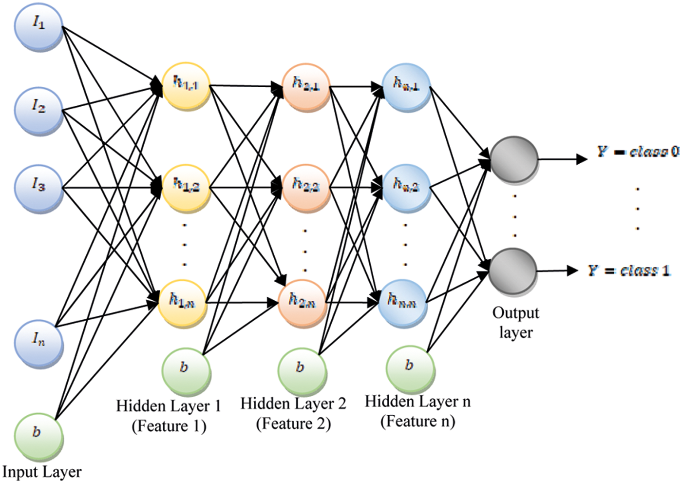
Figure 4: The diagram of DNN structure
The spatial coordinate system (x, y) is transformed into a polar coordinate system (ρ, θ) in the course of its implementation. The polar domain is also discrete in (ρ, θ) terminology, like the spatial domain. When the value of x is different, the rho values change as sinusoidal for a given value of x and y, i.e., a particular point within the spatial domain. Therefore, it gives a sine wave in the accumulator space for each point in the image of the edge detected and there is a specific region that begins to accumulate more votes which means the line with several feature points.
3.4 Proposed Hybrid Deep Neural Network with Modified Crow Search Optimization
The DNN [21] was the simplest and most popular of the distinctive types of neural networks. The data is processed unidirectional in this method. For example, the input layer, the hidden layer, and the output layer are in this framework. The processing elements (PEs) are the image features on each layer of the device. Hubs are referred to as PEs in the scheme. An input node collected by the parameters of the proposed crack detection is shown in Fig. 4. There are weights in each layer in the device. The weight of the sheet is balanced in the preparation process. Network input information sent by heading and prepared before the output layer is achieved. This forward procedure creates the output. An error value can then be calculated if the ideal output is subtracted from the actual output.
The following steps are taken in the implementation of DNN:
Step 1: The input image pixel is initially fed into the first layer of the DNN and it can be interpreted that the outputs of the layer reflect the presence of different low level characteristics such as lines and edges in the image. The input i and secret h units in the DNN structure are started as
When Iuv (input picture parameters) is a symmetrical concept of interaction between the iu input unit and the hidden unit hv; b means the input and hidden units bias, u, v means hidden units.
Step 2: These characteristics are then combined with subsequent layers to quantify the existence of higher level characteristics, e.g., lines are joined into forms that are further combined into sets of forms.
Step 3: In the given visible and hidden units both hidden and input units parallel to each unit and are modified. The dissimilar value is stacked on top of each iteration during the training process and forms a multi-layered model. The values achieved in the DNN layers for the units are divided by the weight of the current network and biases.
Step 4: And, finally, the network is likely to have a crack image or not a crack image, because of all this detail. In the earlier crack detection tasks this profound hierarchy enables DNNs to achieve higher efficiency.
The DNN architecture is divided into 10 hidden layers, sigmoid is used for activation. Sigmoid is the curve formed by S, if y is the net then sigmoid:
For DNN training and a mean square error (MSE), a stochastic gradient (SGD) descent is used for output evaluation and also for fitness of the Modified Crow Search Optimization function (Mcrow). The data are transformed by the DNN’s automated extraction by a cascade of nonlinear transformations, resulting in a representation that is suited for the given problem. The hidden layer, containing parameters to optimize, is common to any transformation. These parameters are improved by Mcrow.
The weight of the network is optimized for the purpose of error rate minimization, thus gives more accuracy in prediction analysis of crack. At each iteration, the weight values are optimized and then train the network. The Mean Square Error (MSE) rate is calculated by
where Di described as Desired value, Pi is the Predicted value, and N is the Number of images. Here, meta-heuristic optimization is used i.e., Mcrow [22–24] to attain the optimal weight value by minimizing the MSE rate. The process involved in Mcrow algorithm is described as follows:
3.6 The Proposed Modified Crow Search Deep Neural Network (Mcrow DNN) Model
In this section the McrowDNN model combines the algorithm of the modifiable crow with the DNN. The input weight and the hidden layer threshold are optimized intelligently by the Mcrow algorithm with the Moore-Penrose generalised reverse matrix in order to measure the output weight value. Then train and construct the optimised DNN model on the image classification data and use the trial set for the early prediction of breakage effects. The McrowDNN algorithm is specifically processed as follows and flow diagram is shown in Fig. 5
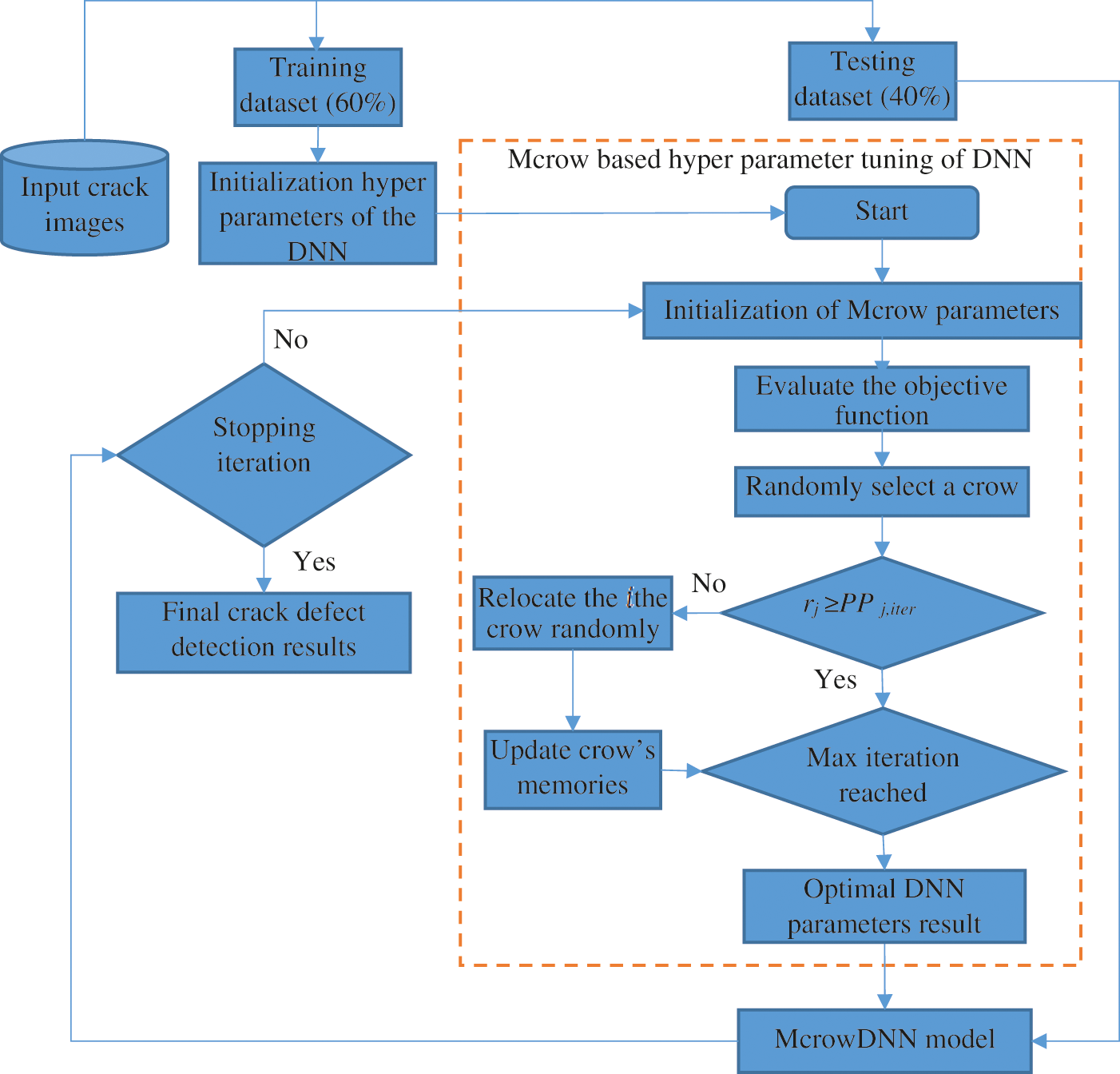
Figure 5: The flow diagram of proposed hybrid McrowDNN algorithm
a. Define the relevant parameters of the Mcrow algorithm and the DNN algorithm, randomly generate a d-dimensional crow population, and then initialize the crow population by mapping based on the chaos method.
b. Initialize the population, randomly generate initial solutions and encode them. The dimension of each solution is × (n + 1) , and the first V × n dimension represents the input weight value. The remaining V dimensions represent hidden layer thresholds, and they are all continuous real numbers.
c. Use the solution obtained in step 2 to decode, obtain the input weight value and the hidden layer threshold, and train the DNN model on the training image data. Note that the solution obtained is actually a vector value, but in the training process it is actually an V × (n + 1)-dimensional matrix, which needs to be converted into a vector form in advance.
d. Calculate the fitness value MSE corresponding to each solution.
e. Increment in iteration as iter = iter + 1.
f. Randomly initialize the position of a flock of N crows in the search space Initialize the memory of each crow
g. Use the features as input weight value and hidden layer threshold value obtained in step 6 to calculate the fitness value corresponding to each solution.
h. A crow j is randomly selected. According to the perception probability PP, if the random number rj is greater than or equal to the perception probability, then the crow i follows the crow j and flies to the memory position of the crow j. If the random number rj is less than the perception probability PP, in order to deceive crow i, crow j will fly to another location according to the new started given in step 9.
i. In the beginning of iterations (for early iterations) for better exploration in the solution space the value of K starts from large number and its value is reduced according to (11) and at the last iterations where the exact searching around the best local optimums is important, the K has the small value. Calculate the K factor as given as follows
j.
k. Select K of the best crows in the population except the current crow (the crow i), updating the position of the crow i by selecting one of these top crows randomly as target (crow j) and use (9) to generate the new position.
l.
a. where, ri and rj are the uniform distributed random numbers in the interval (0, 1) and; fli,iter and PPj,iter are the flight length (fl) of the crow i and perception probability (PP) of the crow j at the iteration iter, respectively. By selecting a small PP, the algorithm performs a search in the area where the current good solution of the j-th crow is located.
m. In Mcrow, the determination of flight length is proposed which leads to select the suitable value of fl with respect to the situations of the crows.
n.
o.
a. where, Disti,j is the vector which contains the distances between the crow i and crow j, Distth is the distance threshold value and flth is a number greater than 2.
p. The current crow position is used as the DNN model parameter and the data is predicted, and the prediction result is converted into a fitness function value and compared with the fitness function value of the memory position of the crow. If it is better than the memory position, the memory m position is updated to the current position.
q.
a. Where xi,iter is the position vector of ith crow in d-dimensional search space and where f(⋅) denotes the objective function.
r. Perform the above steps for all crows, iterate the number of times specified in the above steps, and return the global optimal position as the initial input weight and threshold of the DNN prediction model.
s. Use the new solution obtained in step 13 to train the DNN model and calculate its fitness value.
t. Determine whether the algorithm has reached the maximum number of iterations, if it is satisfied, go to step 13; otherwise, return to step 6 to continue running the algorithm.
u. Decoding from the returned optimal solution can obtain the optimal input weight value, bias value and the threshold value of the hidden layer.
v. Use the trained DNN model to perform classification for test images and record the final crack detection and classification results.
Many experiments were applied to calculate the performance of the proposed system on real crack images which is obtained from Composite Lab, Department of Aerospace Engineering, Indian Institute of Technology, Chennai. A total of 250 images were in collection, and formed as dataset 1 and dataset 2 shown in Figs. 1 and 2 respectively. The dataset 1 contains 125 images (Training images: 88 and Testing images: 37) and dataset 2 contains 98 images (Training images: 69 and Testing images: 29). This proposed McrowDNN algorithm is compared with ANN which is having single hidden layer and RNN which is having 2 hidden layers. A convergence plot of the fitness value vs. the number of iteration for McrowDNN efficiency is presented in Fig. 6. After 6 iterations, the McrowDNN efficiency was almost consistent and a stable optimum point was achieved.
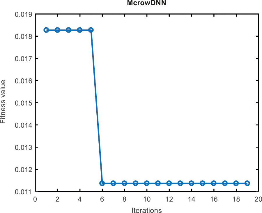
Figure 6: Fitness vs. iteration
After 8 iterations (epochs), the performance of the neural network is plotted on Fig. 7 for dataset 1. At this, the best performance occurs at 2nd iteration and is equal to 0.14477. After 13 iterations (epochs), the performance of the neural network is plotted on Fig. 8 for dataset 2. At this, the best performance occurs at 7th iteration and it is equal to 0.069591. It is evident that the gradient is a locally decreasing function of epochs, which means that if more iteration is involved, the error should be decreased. On the other hand, it can be seen that the validation checks increase when the number of epochs increases.
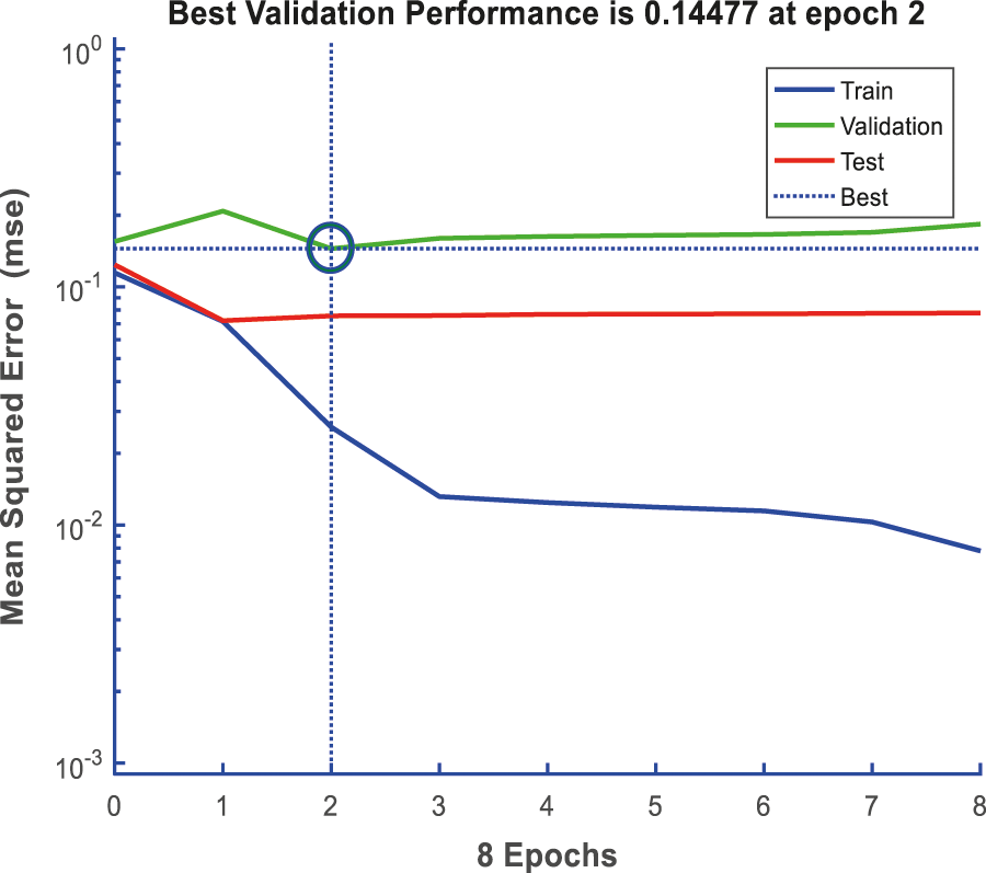
Figure 7: Performance of the DNN for dataset 1
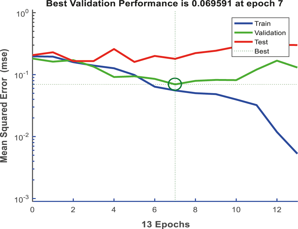
Figure 8: Performance of the DNN for dataset 2
From Figs. 9 and 10, where the error histogram is plotted for dataset 1 and dataset 2 respectively, it is easy to observe that near the zero error (i.e., when the target and output are equal) the training errors for positive difference is comparably higher than that of negative difference.
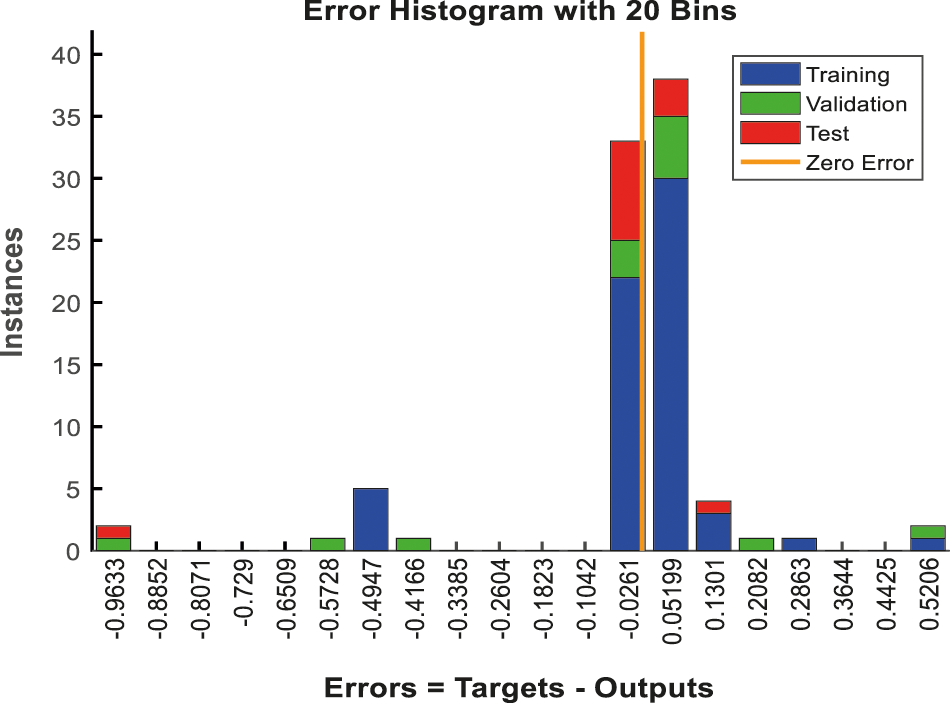
Figure 9: Error histogram for dataset1
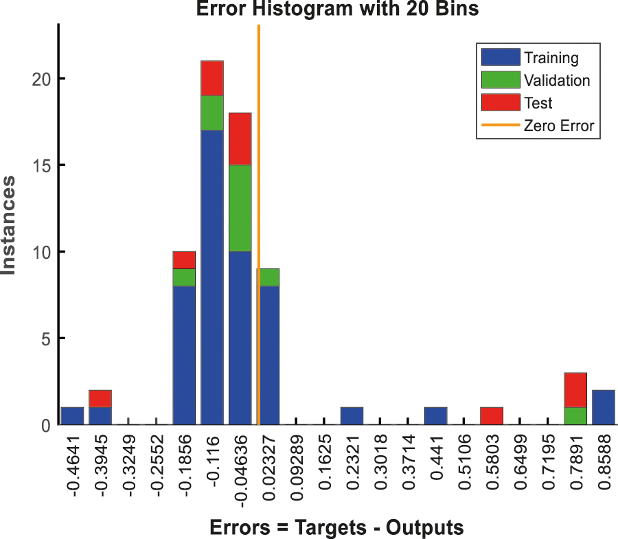
Figure 10: Error histogram for dataset 2
To quantitatively evaluate the performance of different frameworks such as existing ANN and RNN on crack detection database, this work use four common metrics, as shown in equations below which are precision, recall, f-measure and accuracy. All of them are based on four basic components in crack detection: true positive (TP), true negative (TN), false positive (FP), and False negative (FN). TP indicates the number of correctly classified crack pixels, TN indicates the number of correctly classified non-crack pixels, FP indicates the number of mistakenly classified non-crack pixels, and FN indicates the number of mistakenly classified non-crack pixels.
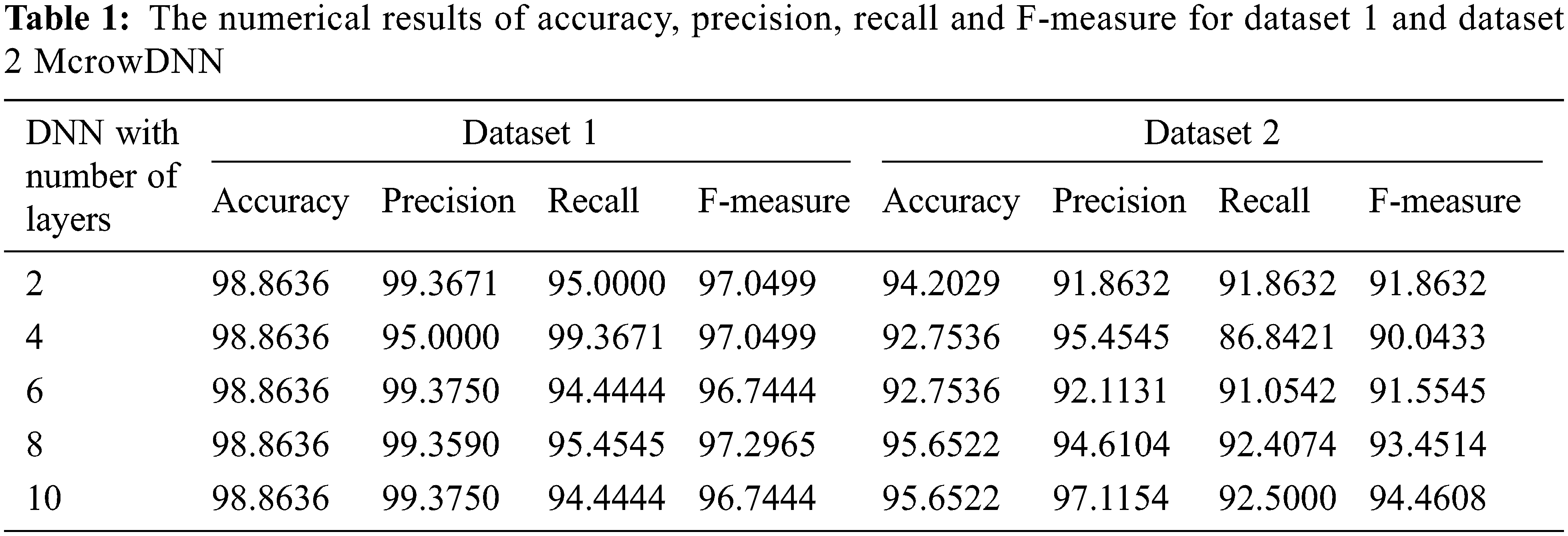
4.3 Comparison Results of Accuracy, Precision, Recall and F-measure for Dataset 1 and Dataset 2-McrowDNN
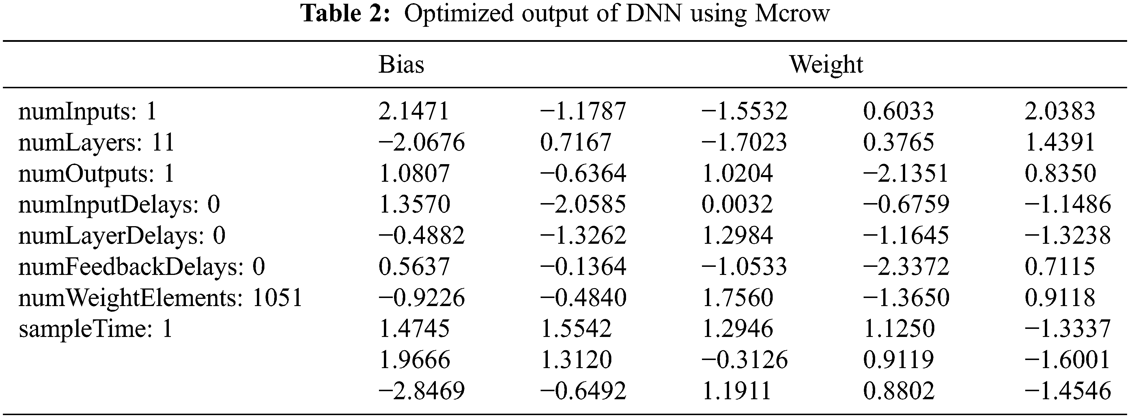
The Figs. 11 and 12 present the Accuracy, precision, recall and f-measure of the McrowDNN for dataset 1 and dataset 2. Hence this discloses all the metrics was noticed, that the McrowDNN produces high results for all four metrics. Furtherly, the detection accuracy, precision, recall and f-measure of the McrowDNN was 98.8636%, 99.3750%, 94.4444% and 96.7444% which was obtained at the layer vale as 10 for dataset 1. Also the detection accuracy, precision, recall and f-measure of the McrowDNN was 95.6522%, 97.1154%, 92.5000% and 94.4608% which was obtained at the layer vale as 10 for dataset 2 as shown in Tab. 1. This results shows that the McrowDNN based crack prediction system can be very helpful to the prediction. The reason is that the proposed DNN is optimized using Mcrow which has the advantage of determining the efficient amount of flight length based on the amount of proximity of crows which helps in a better exploration and thus produce optimal weight, bias and number of layers etc. as shown in Tab. 2.
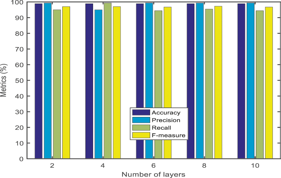
Figure 11: The numerical results of accuracy, precision, recall and F-measure for dataset 1-McrowDNN
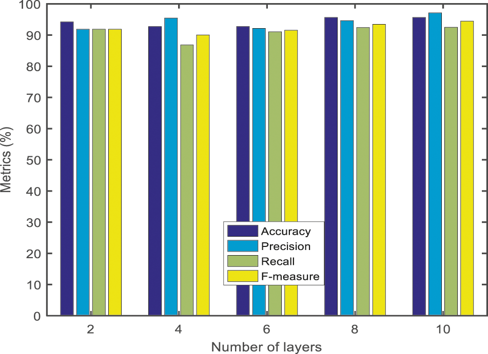
Figure 12: The numerical results of accuracy, precision, recall and F-measure for dataset 2-McrowDNN
4.4 Comparison Results and Discussion
Accuracy
The Fig. 13 presents the Accuracy of the ANN, RNN and McrowDNN. This graph discloses that the McrowDNN was greater than the ANN and RNN plans under the crack image data base. Furtherly, the achieved Accuracy for McrowDNN was 98.8636% for dataset 1 and 94.2029% for dataset 2. This result ensures that the proposed McrowDNN decrease the barriers of detecting crack.
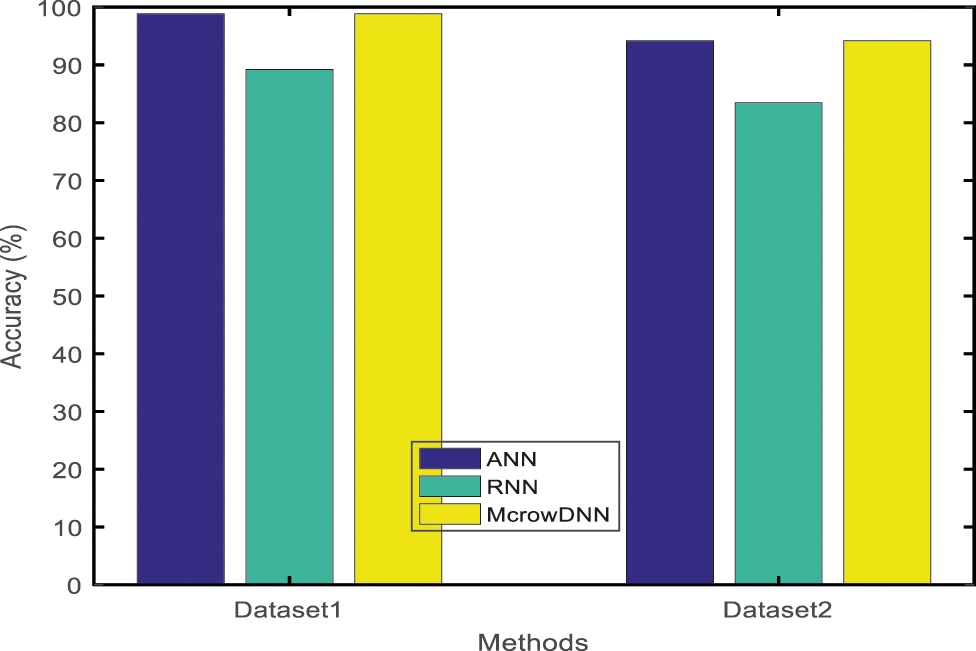
Figure 13: Accuracy comparison results
Precision Rate comparison
In Fig. 14, the graph clarifies the precision for ANN, RNN, and McrowDNN of dataset 1 and dataset 2. The number of images is directly proportional to the precision value. From the above graph, it is studied that the proposed McrowDNN provides higher precision rate at the rate of 98.49522% for dataset 1 and 94.23132% for dataset 2 than the preceding methods. On the other hand, the given experimental results end with the belief that the McrowDNN uses the advantage of faster intersection through the DNN and thus, for the early detection of crack, the McrowDNN acts as a better option.
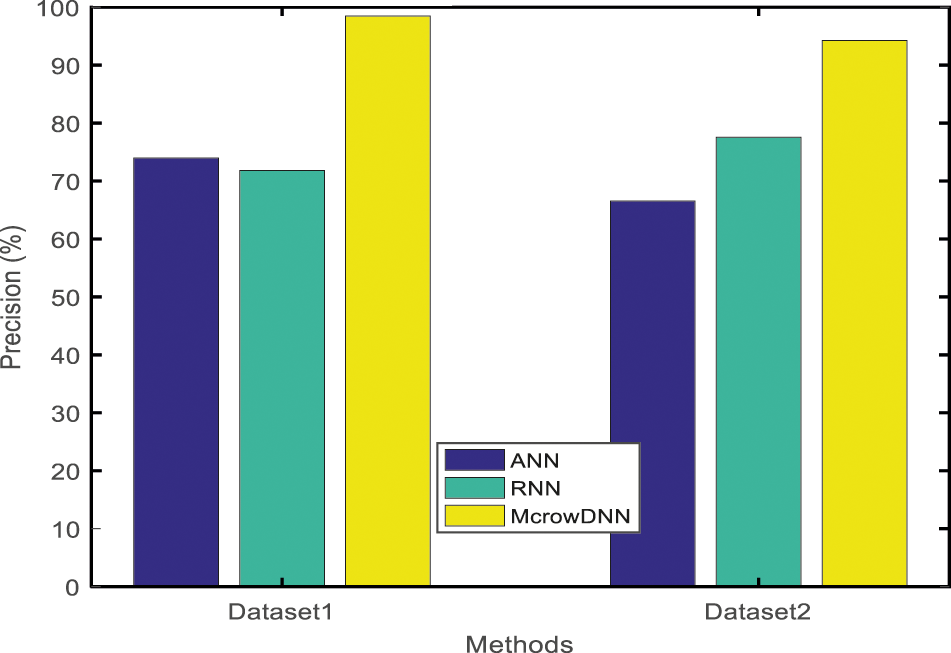
Figure 14: Result of precision rate
Recall Rate Comparison
On the above graph in Fig. 15, while the number of images increases, the recall value also gets increase accordingly and it is clearly evident that the McrowDNN method achieves Recall Rate of 95.74208% for dataset 1 and 90.93338% for dataset 2. Hence from the results it is found that the McrowDNN faster than ANN and RNN framework, thus their precision of the neural network stays saturated.
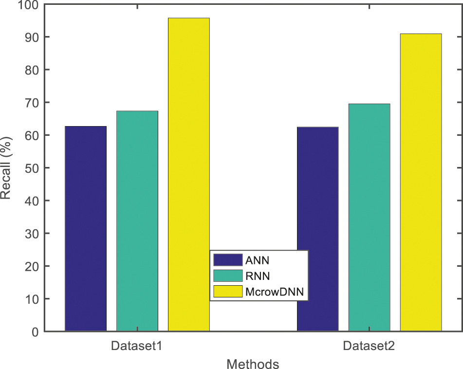
Figure 15: Result of recall rate
F-measure Rate Comparison
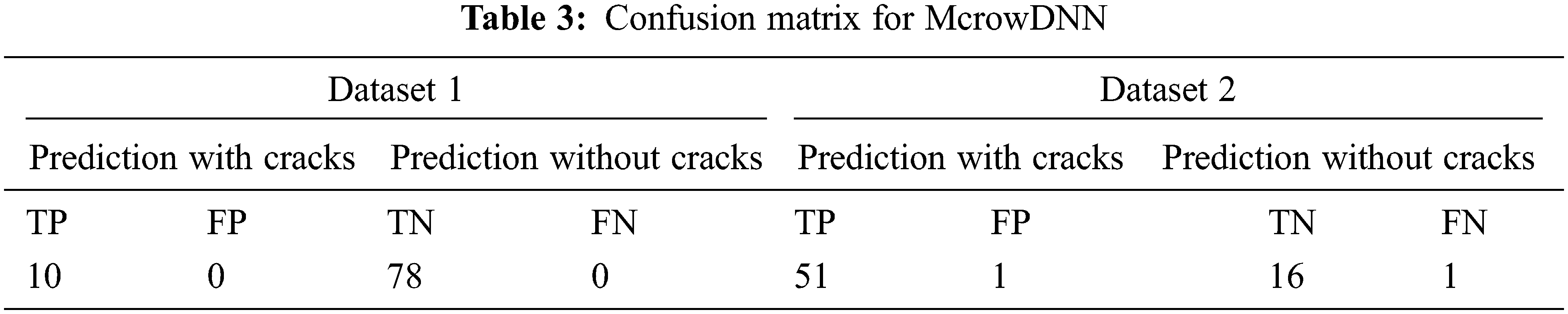
In the given Fig. 16, the graph shows the F-measure rate for ANN, RNN and McrowDNN. The McrowDNN gives 96.97702% for dataset 1 and 92.27464% for dataset 2 and it achieves a better F-measure rate compared to other two preceding methods. It is found that the proposed McrowDNN accomplish a good accuracy results with 10 numbers of layers and it outperforms than the existing methods. The performance of the classification model is further analyzed using confusion matrix. The confusion matrix obtained from the McrowDNN algorithm is shown in Tab. 3 for dataset 1 and 2 respectively.
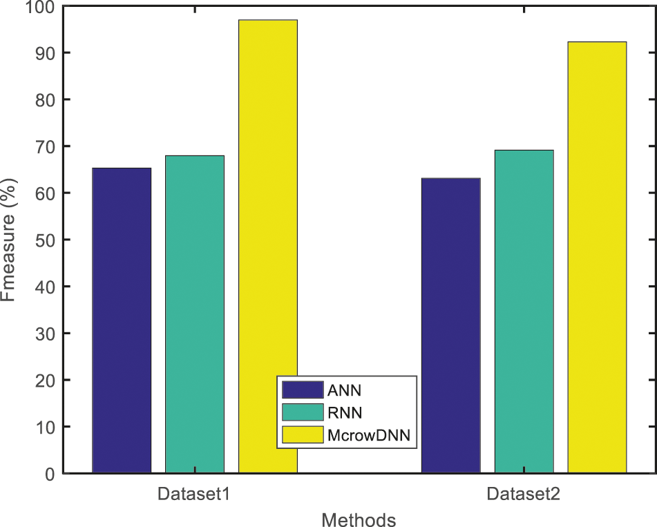
Figure 16: Result of F-measure rate
This work proposed a method for the detection of cracks in composite material images with McrowDNN which is particularly powerful in the classification of images because it can learn certain features automatically from the input images. This proposed McrowDNN is an automated detection system where the features of manually annotated picture patches are automatically done. The Mcrow has been applied to simplify the DNN structure to obtain better solutions with timing concern. From the test results, it has been inferred that the proposed system is able to detect cracks in composite materials images. In future, the proposed work can be improved by adding more pictures with the current database to do comparison tests under different scale of composite images with more types of with defects and the study will be further extended to measure the length and depth of the cracks in composite material to assess the degree of severity.
Acknowledgement: The authors like to acknowledge and thank the management, director, principal and Head of CSE and ECE department for providing facilities to carry out the research work.
Funding Statement: The authors received no specific funding for this research work.
Conflicts of Interest: The authors declare that they have no conflicts of interest to report regarding the present research work.
1. A. Kapadia, “Non-destructive testing of composite materials,” [Online]. Available: https://avaloncsl.files.wordpress.com/2013/01/ncn-best-practice-ndt.pdf, 2007. [Google Scholar]
2. K. K. Chawla, “Composite materials science and engineering,” in Proc. 3rd Edition in Springer Science Business Media, pp. 1–552, 2012. http://opac.lib.idu.ac.id/unhan-ebook/assets/uploads/files/28457-composite-materials-science-and-engineering-by-krishan-k.-chawla-auth.-z-lib.org-.pdf. [Google Scholar]
3. C. Boller, F. K. Chang and Y. Fujino, Encyclopedia of Structural Health Monitoring. Hoboken, New Jersey, United States: John Wiley and Sons. pp. 1–2960, 2009. [Google Scholar]
4. H. Towsyfyan, A. Biguri, R. Boardman and T. Blumensath, “Successes and challenges in non-destructive testing of aircraft composite structures,” Chinese Journal of Aeronautics, vol. 33, no. 3, pp. 771–991, 2020. [Google Scholar]
5. G. Deepak, R. Joel, S. Sundaram and A. Khanna, “Usability feature extraction using modified crow search algorithm: A novel approach,” Neural Computing and Applications, vol. 32, pp. 10915–10925, 2020. [Google Scholar]
6. Y. Gong, H. Shao, J. Luo and Z. Li, “A deep transfer learning model for inclusion defect detection of aeronautics composite materials,” Composite Structures, vol. 252, pp. 112681, 2020. [Google Scholar]
7. M. Rautela and S. Gopalakrishnan, “Ultrasonic guided wave based structural damage detection and localization using model assisted convolutional and recurrent neural networks,” Expert Systems with Applications, vol. 167, no. 1, pp. 114189, 2020. [Google Scholar]
8. D. W. Abueidda, M. Almasri, R. Ammourah, U. Ravaioli, I. M. Jasiuk et al., “Prediction and optimization of mechanical properties of composites using convolutional neural networks,” Composite Structures, vol. 227, no. 1, pp. 111264, 2019. [Google Scholar]
9. T. Guo, L. Wu, C. Wang and Z. Xu, “Damage detection in a novel deep-learning framework: A robust method for feature extraction,” Structural Health Monitoring, vol. 19, no. 2, pp. 424–442, 2019. [Google Scholar]
10. V. Ewald, X. Goby, H. Jansen, R. Groves and R. Benedictus, “Incorporating inductive bias into deep learning: A perspective from automated visual inspection in aircraft maintenance,” in Proc. 10th Int. Symp. on NDT in Aerospace, Dresden, 2018. [Google Scholar]
11. B. Hyun-Tae, S. Park and H. Jeo, “Defect identification of composites via thermography and deep learning techniques,” Composite Structures, vol. 246, pp. 112405, 2020. [Google Scholar]
12. A. Khan, K. Dae-Kwan, S. C. Lim and H. S. Kim, “Structural vibration-based classification and prediction of delamination in smart composite laminates using deep learning neural network,” Composites Part B: Engineering, vol. 161, pp. 586–594, 2019. [Google Scholar]
13. A. Katunin, K. Dragan and M. Dziendzikowski, “Damage identification in aircraft composite structures: A case study using various non-destructive testing techniques,” Composite Structures, vol. 127, pp. 1–9, 2015. [Google Scholar]
14. T. A. Carr, M. D. Jenkins, M. I. Iglesias, T. Buggy and G. Morison, “Road crack detection using a single stage detector based deep neural network,” in Proc. IEEE Workshop on Environmental, Energy, and Structural Monitoring Systems (EESMS), Italy, 2018. [Google Scholar]
15. S. Albawi, T. A. Mohammed and S. Al-Zawi, “Understanding of a convolutional neural network,” in Proc. 2017 Int. Conf. on Engineering and Technology (ICET), Turkey, 2017. [Google Scholar]
16. J. Gua, Z. Wang, J. Kuen, L. Ma, A. Shahroudy et al., “Recent advances in convolutional neural networks,” Pattern Recognition, vol. 77, pp. 354–377, 2018. [Google Scholar]
17. H. H. Aghdam and E. J. Heravi, “Guide to convolutional neural networks,” [Online]. Available: https://link.springer.com/book/10.1007/978-3-319-57550-6, 2017. [Google Scholar]
18. N. Nausheen, A. Seal, P. Khanna and S. Halder, “A FPGA based implementation of sobel edge detection,” Microprocessors and Microsystems, vol. 56, pp. 84–91, 2018. [Google Scholar]
19. M. A. Hannan, W. A. Zaila, M. Arebey, R. A. Begum and H. Basri, “Feature extraction using hough transform for solid waste bin level detection and classification,” Environmental Monitoring and Assessment, vol. 186, no. 9, pp. 5381–5391, 2014. [Google Scholar]
20. M. Priyanka and B. B. Chaudhuri, “A survey of hough transform,” Pattern Recognition, vol. 48, no. 3, pp. 993–1010, 2015. [Google Scholar]
21. A. Canziani, A. Paszke and E. Culurciello, “An analysis of deep neural network models for practical applications,” [Online]. Available: https://arxiv.org/abs/1605.07678, 2016. [Google Scholar]
22. F. Mohammadi and H. Abdi, “A modified crow search algorithm (Mcrow) for solving economic load dispatch problem,” Applied Soft Computing, vol. 71, pp. 51–65, 2018. [Google Scholar]
23. P. Díaz, M. Pérez-Cisneros, E. Cuevas, O. Avalos, J. Gálvez et al., “An improved crow search algorithm applied to energy problems,” Energies, vol. 11, no. 3, pp. 571, 2018. [Google Scholar]
24. L. D. S. Coelho, C. Richter, V. C. Mariani and A. Askarzadeh, “Modified crow search approach applied to electromagnetic optimization,” in Proc. IEEE Conf. on Electromagnetic Field Computation (CEFC), Miami FL USA, 2016. [Google Scholar]
 | This work is licensed under a Creative Commons Attribution 4.0 International License, which permits unrestricted use, distribution, and reproduction in any medium, provided the original work is properly cited. |