DOI:10.32604/iasc.2022.025214
| Intelligent Automation & Soft Computing DOI:10.32604/iasc.2022.025214 | |
| Article |
Bayesian Convolution for Stochastic Epidemic Model
1Department of Statistics, Faculty of Mathematics and Natural Sciences, Universitas Halu Oleo, Kendari, 93232, Indonesia
2Department of Statistics, Faculty of Mathematics and Natural Sciences, Universitas Negeri Makassar, Makassar, 90223, Indonesia
3Department of Mathematics and Statistics, College of Sciences, Taif University, Taif, 21944, Saudi Arabia
4Department of Statistics, Mathematics, and Insurance, Faculty of Commerce, Tanta University, Egypt
5Department of Economics and Finance, College of Business Administration, Taif University, Taif, 21944, Saudi Arabia
6Department of Mathematics, College of Sciences and Arts, Najran University, Najran, 66445, Saudi Arabia
*Corresponding Author: Mukhsar. Email: mukhsar.mtmk@uho.ac.id
Received: 16 November 2021; Accepted: 14 January 2022
Abstract: Dengue Hemorrhagic Fever (DHF) is a tropical disease that always attacks densely populated urban communities. Some factors, such as environment, climate and mobility, have contributed to the spread of the disease. The Aedes aegypti mosquito is an agent of dengue virus in humans, and by inhibiting its life cycle it can reduce the spread of the dengue disease. Therefore, it is necessary to involve the dynamics of mosquito's life cycle in a model in order to obtain a reliable risk map for intervention. The aim of this study is to develop a stochastic convolution susceptible, infective, recovered-susceptible, infective (SIR-SI) model describing the dynamics of the relationship between humans and Aedes aegypti mosquitoes. This model involves temporal trend and uncertainty factors for both local and global heterogeneity. Bayesian approach was applied for the parameter estimation of the model. It has an intrinsic recurrent logic for Bayesian analysis by including prior distributions. We developed a numerical computation and carry out simulations in WinBUGS, an open-source software package to perform Markov chain Monte Carlo (MCMC) method for Bayesian models, for the complex systems of convolution SIR-SI model. We considered the monthly DHF data of the 2016–2018 periods from 10 districts in Kendari-Indonesia for the application as well as the validation of the developed model. The estimated parameters were updated through to Bayesian MCMC. The parameter estimation process reached convergence (or fulfilled the Markov chain properties) after 50000 burn-in and 10000 iterations. The deviance was obtained at 453.7, which is smaller compared to those in previous models. The districts of Wua-Wua and Kadia were consistent as high-risk areas of DHF. These two districts were considered to have a significant contribution to the fluctuation of DHF cases.
Keywords: Bayesian; convolution; dengue hemorrhagic fever; MCMC; SIR-SI model; stochastic; temporal trend
Epidemic diseases are fatal infectious diseases, for example measles, dengue fever, malaria, HIV/AIDS, tuberculosis, influenza, etc. To reduce the threat of virus spread, various strategies can be used using epidemic models. Many studies have been applied to the investigation of infectious diseases, including nonlinear differential equation models to describe nonlinear incidence rates and relative risk analysis [1–4]. Epidemic cases have played an important role as one of the causes of poverty, misery, and death for humanity for centuries. In recent years, statistical models and their computations have been able to explain more formal epidemic studies. Several types of epidemic models using various techniques have been proposed such as the susceptible,infected,removed (SIR) model to understand the evolution of complex infectious diseases to predict the impact of public health programs [5].
Dengue Hemorrhagic Fever (DHF) is a tropical disease. It has become a plague and always attacks densely populated urban communities every year. The transmission process is influenced by several factors, such as environment, climate change, and uncertainty or mobility of people, e.g., [5,6]. The agent of DHF is Aedes aegypti mosquitoes to humans through bites. The Aedes aegypti mosquitoes carry the dengue virus to humans. A common symptom of dengue virus infection is fever. It is often ignored and it results in a fatal end.
One way to reduce the DHF spread is to break the Aedes aegypti mosquitoes life cycle. However, it requires detailed calculation as its population fluctuates depending on the environmental characteristics that cannot be controlled. Besides, characteristic differences of locations lead to the complexity in controlling the spread of dengue disease. These characteristics of location are subject to change and affected by seasons. The mobility of people also plays an important role in DHF cases. Therefore, a comprehensive model that accommodates all conditions mentioned above is needed. Several statistical studies have been undertaken to analyze DHF cases spatially and temporally. For example, the Bayesian zero-inflated spatial-temporal Poisson model by [7–10] to analyze the relative risk of dengue cases. Those models accommodated the environmental ecological factors and two random effects (local and global heterogeneity) to represent the actual mobility of people. However, the studies did not consider the cross-infection dynamics between humans and the Aedes aegypti mosquitoes. The dynamics of the cross-infection relationship is not reflected in the modeling.
Other studies employed stochastic processes to represent the cross-infection relationship between humans and mosquitoes, e.g., [11,12]. A more recent study is the work of [13] which is describing the stochastic process of cross-infection between humans and mosquitoes. This research used a global random effect, but it cannot represent the pattern of overall distribution. Humans as hosts are divided into three classes, namely susceptible, infected, and recovered hosts. Meanwhile, mosquitoes as vector are divided into two classes, namely susceptible and infective vectors. The model is known as a stochastic SIR-SI model. Our research develops a stochastic SIR-SI model that accommodates two local and global random effects by involving the temporal trends as well as the spatial-temporal term. This is called the Bayesian stochastic convolution SIR-SI model with the temporal trend. Detailed descriptions of the local and global heterogeneity components can be seen in [8]. This model is expected to be used in public health protection by quickly detecting and responding to outbreaks of DHF cases, which poses a growing threat to human health.
The Bayesian approach is especially suitable for epidemic modeling contexts, such as this stochastic SIR-SI model with the temporal trend, because the model parameters have a certain distribution across the population. To date, virtually all of the literature on Bayesian statistical inference uses numerical techniques such as Markov Chain Monte Carlo (MCMC) for epidemic modeling [14]. Thus, in this model, the Bayesian paradigm is used, which can overcome a more complex model. In this article, we develop the model [9] by adding the uncertainty factor and the temporal trend. We compiled two models, the first model is containing global uncertainty and the second model accommodates local and global uncertainty as well as temporal trend. The performances of these two models are using monthly DHF data in 10 districts of Kendari City-Indonesia for the 2016–2018 periods.
The structure of this paper is as follows. In Section 2, we present a schema of cross-infection model. In Section 3, we present several types of models using the Bayesian stochastic SIR-SI model. To obtain estimated parameters of model. In Section 4, we illustrate some simulation experiments and determine the best model using monthly data for 10 districts of Kendari City-Indonesia, for the 2016–2018 periods.
The cross-infection diagram of the DHF spread between host and vector is based on the disease status. The host is divided into three classes, namely susceptible host or
The stochastic SIR-SI model is generally used to study DHF transmission [13]. All individuals in the population are equally probable to have contact with other individuals [4,15]. In real conditions, the contact patterns between people are more heterogeneous. This results in heterogeneous patterns of disease spread. Consequently, a stochastic model can be used to determine the pattern of infection transmission by assuming that the number of individuals is considered a random variable and has a certain distribution [16]. Stochastic models can easily be examined from a Bayesian point of view, for example [17–19].
In this paper, for s = 1, 2, …, S = study regions, and t = 1, 2, …, T = time periods, each notation showed in Fig. 1 is defined as follows.
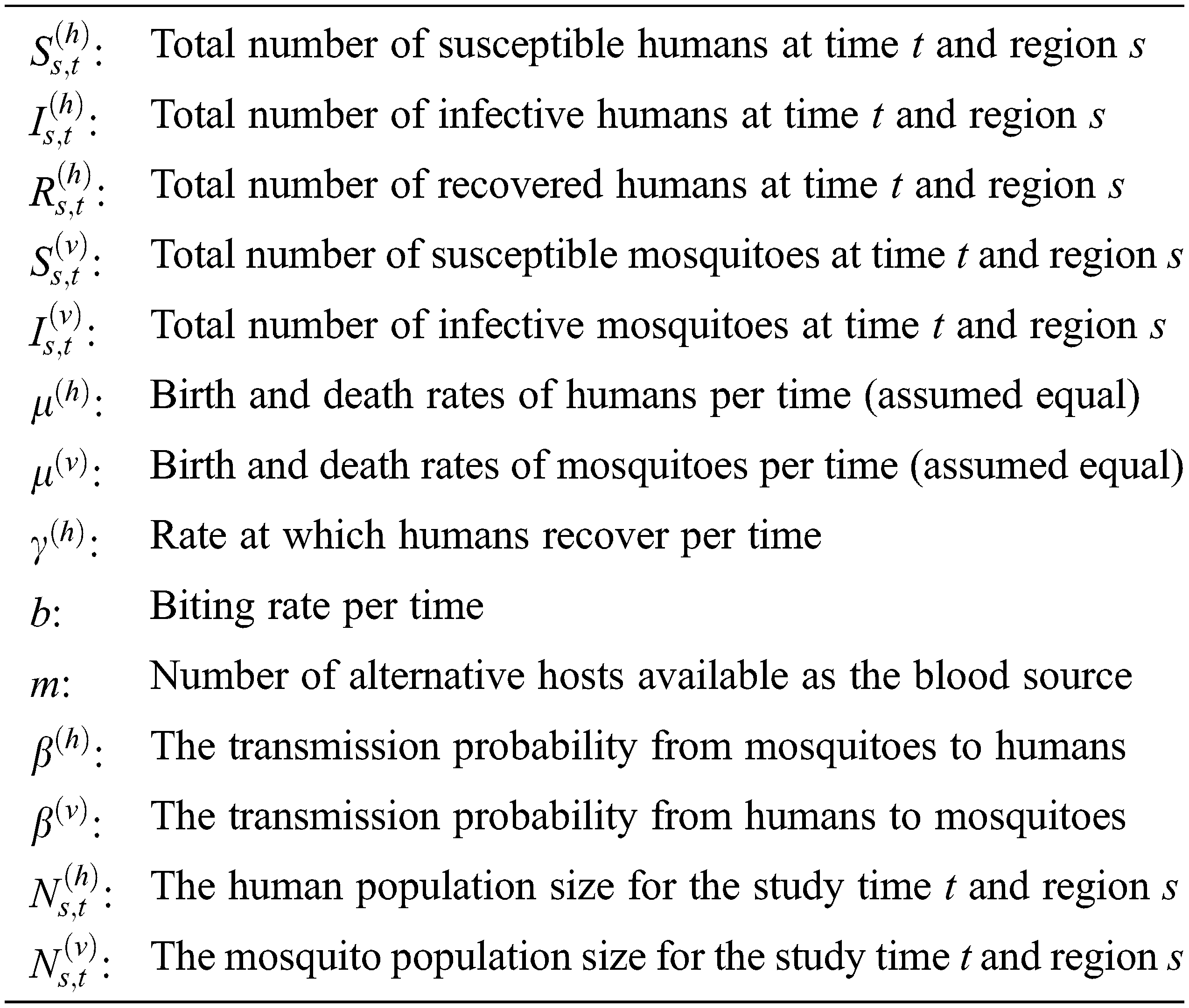
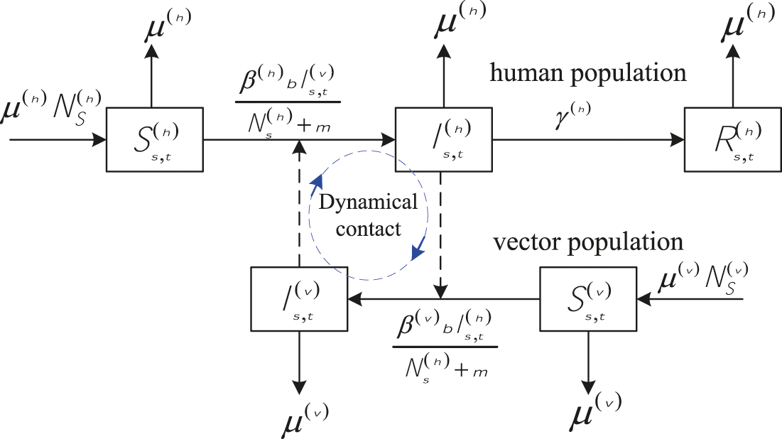
Figure 1: The SIR-SI schema (adopted from [13])
The susceptible, infected and recovered host at time
The system of ordinary differential Eq. (1) has the same form as that used by [13]. The system is used to provide a link to the stochastic process. In this study,
3 Temporal Trend Convolution Stochastic SIR-SI Model
The stochastic SIR-SI model represents the DHF epidemic spread, e.g., [13,23]. This model is useful for analyzing and mapping the DHF risk cases spatially and temporally, by accommodating the random global heterogeneity
The structure of the system (2) contains the global heterogeneity random effect
The parameters in (2) and (3) are estimated using the MCMC Bayesian approach. The Bayesian paradigm using a distribution approach is powerful in overcoming complex modeling. In Bayesian modeling, the observation data is assumed to have a certain distribution. The parameters have uncertainty properties and, then, require prior distribution [7]. The process for obtaining posterior distribution requires the likelihood function and the prior distribution. Several types of prior distributions are known in Bayesian modeling, such as conjugate prior, non-conjugate prior, informative prior, and non-informative prior [23].
We use hyper prior derived from the prior distribution family to obtain precise parameter estimates of models (2) and (3). The prior of host birth
the
4 Application for Relative Risk Estimation
This section demonstrates the numerical process to obtain estimated parameters of the model (2) and model (3) as described in Section 3. Both models are applied to the same data set of the monthly 10 districts DHF cases of Kendari, Indonesia, for the 2016–2018 periods. The ten districts are Mandonga, Baruga, Puuwatu, Kadia, Wua-Wua, Poasia, Abeli, Kambu, Kendari, and Kendari Barat. The population density of Kendari is around 1,364 people per km2. The highest rainfall is around 3000 mm3–3030 mm3 and it usually occurs in early January to April. The data set of rainfall was collected from BMKG Kendari, Indonesia. The highest rainfall usually supports the proliferation of Aedes aegypti mosquitoes.
The parameters of models are estimated and analyzed using open-source software WinBUGS (See Fig. 2). It is a statistical package designed to carry out a wide variety of Bayesian models [7]. The package provides some models along with their corresponding deviance for a given data set. The best model is that with the smallest deviance and it is used to analyze the relative and mapping risk of DHF cases. The results of relative risk estimation based on the best model are presented in graphs to show overall DHF relative risks for each district in Kendari. Dengue mosquito data is estimated according to new infective mosquito data
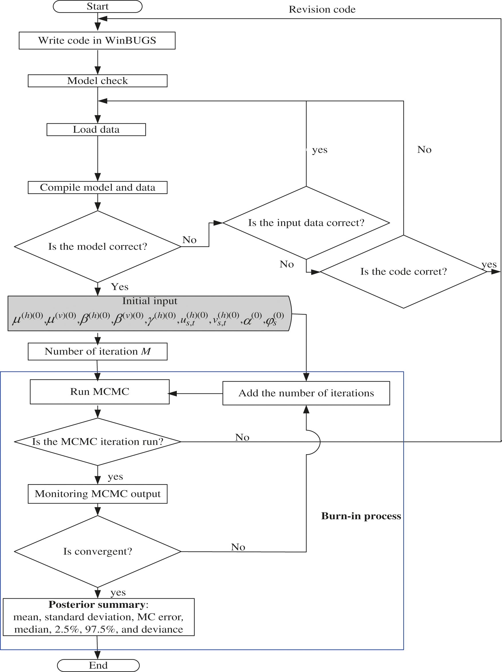
Figure 2: Flowchart for estimation parameter of the models
The parameter estimation was updated throughout iterations via Bayesian MCMC Gibbs Sampler based on its full conditional distribution. Initial values of
are based on our experience. The parameter estimation processes of the models achieved convergence in 50000 burn-in 10000 iterations and fulfilled the Markov Chain properties [9]. This is confirmed by the sample of the history, density, and auto correlation plots. The iteration process showed that the estimated parameters lied in the same zone. In another hand, iteration n + 1 is equivalent to iteration n (see Fig. 3).
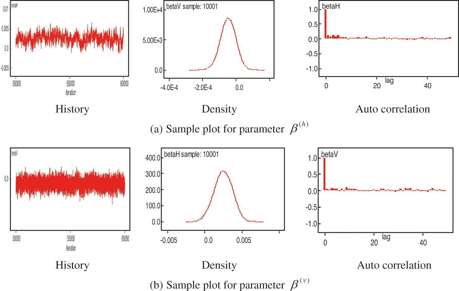
Figure 3: Samples of parameter estimation of the model (3), 50000 burn-in 10000 iterations
In Fig. 3, we show the numerical process of estimating parameters, for example
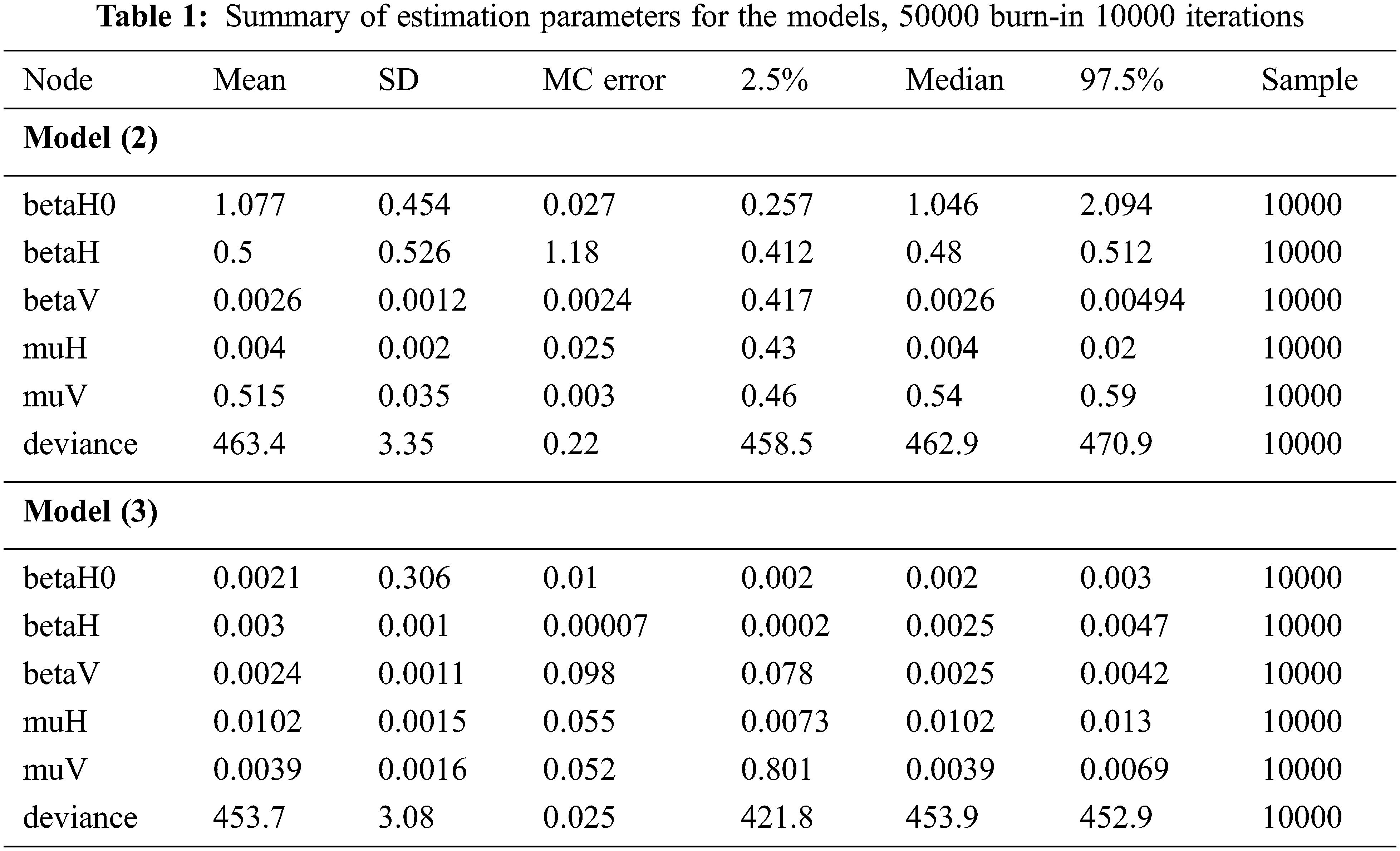
The stochastic model (3) has smaller deviance 453.7 and, therefore, this model is the best one. Thus, this model (3) was used to analyze the DHF mapping relative risk. The DHF cases in Kendari City was fluctuating from January to May each year. During this period, the DHF cases showed that Kadia and Wua-Wua districts were consistent as the highest locations of DHF cases. Other locations around these two districts, such as Mandonga, Puuwatu, Baruga, and Kendari Barat are fluctuating temporally. Therefore, these two districts need special treatment to reduce the DHF outbreak in Kendari City. The monthly dynamics of DHF risk in Kendari city, for the January–May period each year.The dynamics of DHF risk visualization in Kendari City are described in the mapping in Fig. 4
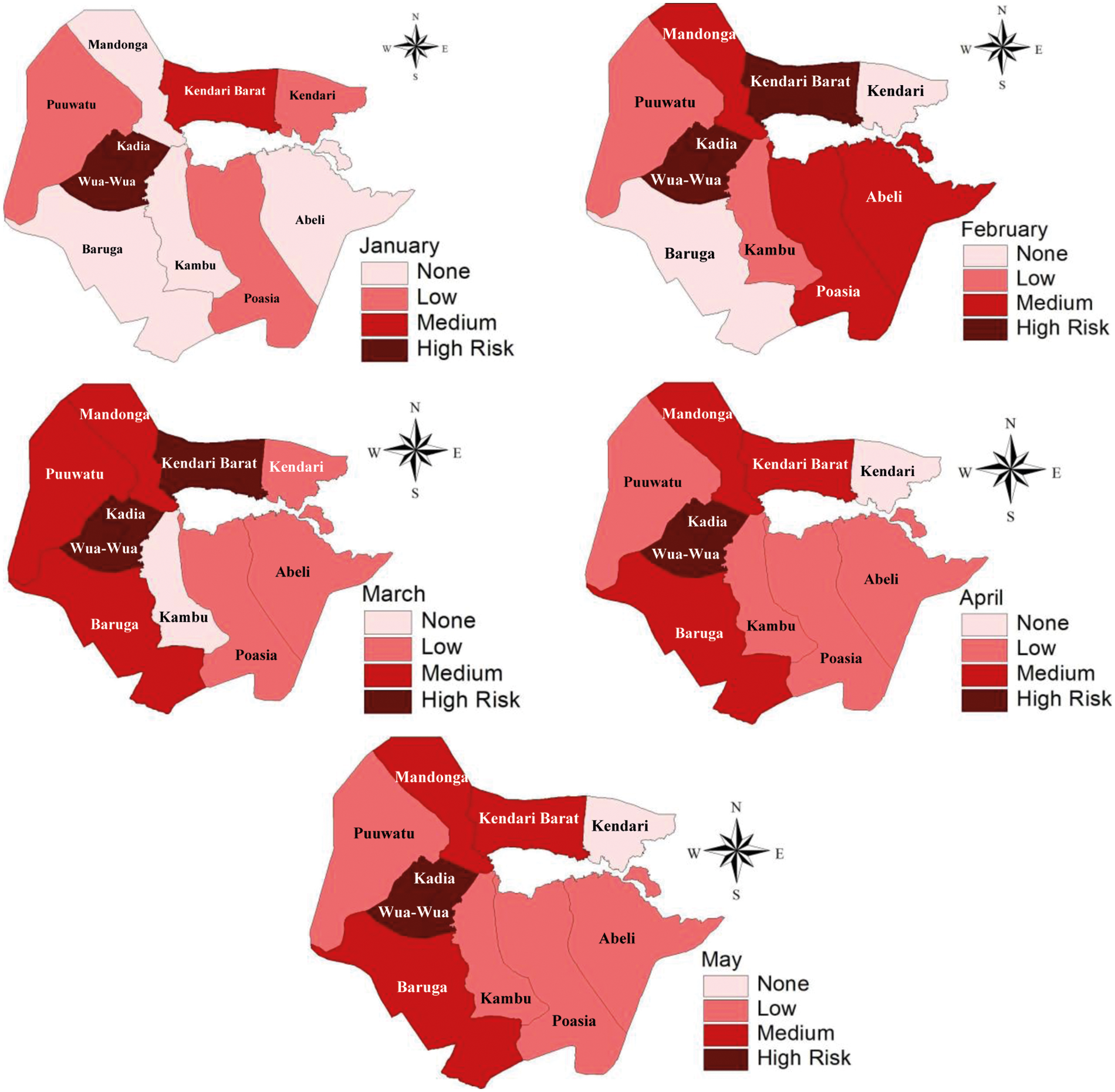
Figure 4: Relative risk DHF mapping using the model (3)
We have developed a stochastic convolution SIR-SI model of the dynamic relationship between humans and Aedes aegypti mosquitoes. This model involves temporal trend factors due to the temporal dynamics of DHF cases. The model also accommodates the uncertainty factors, which are the local and global heterogeneity. The Bayesian approach becomes the choice for parameter estimations of the models. We have demonstrated the models using DHF monthly data for 10 districts of Kendari-Indonesia for the 2016–2018 periods. The parameter estimations of the models were updated via Bayesian MCMC Gibbs Sampler based on its full conditional distribution. The parameter estimation processes of the models achieved convergences after 50000 burn-in 10000 iterations and fulfilled the Markov Chain properties. Our model is considered as the best one because of its smallest deviance 453.7. The results of our model show that Wua-Wua and Kadia districts were consistent as high-risk areas of DHF. In these two districts, the DHF cases exceeded the common fluctuations in other districts, such as Mandonga, Puuwatu, Baruga, and Kendari Barat.
We have used numerical processes to determine the convolution SIR-SI model solution. The convolution SIR-SI model is an ordinary nonlinear differential equation that cannot be solved analytically. Therefore, it was transformed into a discrete form using the Euler method. This method effectively converts the continuous-time of the convolution SIR-SI model into discrete-time. The numerical process has been able to provide useful information for the stochastic process of the nonlinear convolution SIR-SI system. This process has provided information about SIR and SI populations to estimate relative risk. This analysis contributes to the prevention and control of infectious diseases.
In general, closed-form expressions for the posterior distributions are often intractable for these complex models and Markov Chain Monte Carlo (MCMC) algorithms can be used for inference, although this approach can be computationally demanding. However, a new technique based on the integrated nested Laplace approximation (INLA). Most results show that INLA is much more computationally efficient than the other and the precision parameter estimates in both methods are equivalent. For future studies, we will consider the dynamics of ecological factors to formulate several spatio temporal hierarchical models either separately or simultaneously in a small area with INLA.
Acknowledgement: The authors gratefully acknowledge to the Department of Health, BPS, and BMKG of Kendari-Indonesia for their permission to use their observation data in this study.
Funding Statement: The authors received no specific funding for this study.
Conflicts of Interest: The authors declare that they have no conflicts of interest to report regarding the present study.
1. U. Fatima, D. Baleanu, N. Ahmed, S. Azam, A. Raza et al., “Numerical study of computer virus reaction diffusion epidemic model,” Computers Materials & Continua, vol. 66, no. 3, pp. 3183–3194, 2021. [Google Scholar]
2. K. E. Macías-Díaz, A. Raza, N. Ahmed and M. Rafiqe, “Analysis of a nonstandard computer method to simulate a nonlinear stochastic epidemiological model of coronavirus-like diseases,” Computer Methods and Programs in Biomedicine, vol. 2021, no. 204, pp. 1–10, 2021. [Google Scholar]
3. A. Raza, M. Rafiq, D. Baleanu, M. S. Arif, M. Naveed et al., “Competitive numerical analysis for stochastic HIV/AIDS epidemic model in a two-sex population,” IET Systems Biology, vol. 3, no. 6, pp. 305–315, 2019. [Google Scholar]
4. A. Raza, M. S. Arif and M. Rafiq, “A reliable numerical analysis for stochastic dengue epidemic model with incubation period of virus,” Advances in Difference Equations, vol. 2019, no. 32, pp. 1–19, 2019. [Google Scholar]
5. L. Esteva and C. Vargas, “Analysis of a dengue disease transmission model,” Mathematical Biosciences, vol. 150, no. 2, pp. 131–151, 1998. [Google Scholar]
6. Mukhsar, “The Bayesian zero-inflated negative binomial (t) spatio-temporal model to detect an endemic DHF location,” Far East Journal of Mathematical Sciences, vol. 109, no. 2, pp. 357–372, 2018. [Google Scholar]
7. B. A. Lawson, Bayesian Disease Mapping: Hierarchical Modeling in Spatial Epidemiology. Chapman & Hall: CRC Press, 2008. [Online]. Available at: https://www.routledge.com/Bayesian-Disease-Mapping-Hierarchical-Modeling-in-Spatial-Epidemiology/Lawson/p/book/9780367781224. [Google Scholar]
8. Mukhsar, B. Abapihi, A. Sani, E. Cahyono and P. Adam, “Extended convolution model to Bayesian spatio-temporal for diagnosing DHF endemic locations,” Journal of Interdisciplinary Mathematics, vol. 19, no. 2, pp. 233–244, 2016. [Google Scholar]
9. A. Sani, B. Abapihi, M. Mukhsar and K. Kadir, “Relative risk analysis of dengue cases using convolution extended into spatio-temporal model,” Journal of Applied Statistics, vol. 42, no. 11, pp. 2509–2519, 2015. [Google Scholar]
10. Mukhsar, N. Iriawan, B. S. S. Ulama and S. Sutikno, “New look for DHF relative risk analysis using Bayesian poisson-lognormal 2-level spatio-temporal,” International Journal of Applied Mathematics and Statistics, vol. 47, no. 17, pp. 39–46, 2013. [Google Scholar]
11. D. Clancy, “A stochastic SIS infection model incorporating indirect transmission,” Journal of Applied Probability, vol. 42, no. 3, pp. 726–737, 2005. [Google Scholar]
12. L. Knorr-Held and J. Besag, “Modelling risk from a disease in time and space,” Statistics in Medicine, vol. 17, no. 18, pp. 2045–2060, 1998. [Google Scholar]
13. N. A. Samat and D. F. Percy, “Vector-borne infectious disease mapping with stochastic difference equations: An analysis of dengue disease in Malaysia,” Journal of Applied Statistics, vol. 39, no. 9, pp. 2029–2046, 2012. [Google Scholar]
14. P. D. O’Neil, “A tutorial introduction to Bayesian inference for stochastic epidemic models using Markov chain Monte Carlo methods,” Mathematical Biosciences, vol. 180, no. 1–2, pp. 103–114, 2002. [Google Scholar]
15. P. Pongsumpun, K. Patanarapelert, M. Sripom, S. Varamit and I. M. Tang, “Infection risk to travellers going to dengue fever endemic regions,” Southeast Asian Journal of Tropical Medicine and Public Health, vol. 35, no. 1, pp. 155–159, 2004. [Google Scholar]
16. C. L. Addy, I. M. Jr. Longini and M. Haber, “A generalized stochastic model for the analysis of infectious disease final size data,” Biometrics, vol. 47, no. 3, pp. 961–974, 1991. [Google Scholar]
17. L. Bernardinelli, D. G. Clayton, C. Pascutto, C. Montomoli, M. Ghislandi et al., “Bayesian analysis of space-time variation in disease risk,” Statistics in Medicine, vol. 14, no. 21–22, pp. 2433–2443, 1995. [Google Scholar]
18. D. Boehning, E. Dietz and P. Schlattmann, “Space-time mixture modelling of public health data,” Statistics in Medicine, vol. 19, no. 17–18, pp. 2333–2344, 2000. [Google Scholar]
19. D. Clancy and P. D. O’Neill, “Bayesian estimation of the basic reproduction number in stochastic epidemic models,” Bayesian Analysis, vol. 3, no. 4, pp. 737–758, 2008. [Google Scholar]
20. E. Cahyono, Mukhsar and P. Elastic, “Dynamics of knowledge dissemination in a four-type population society,” Far East Journal of Mathematical Sciences, vol. 102, no. 6, pp. 1065–1076, 2017. [Google Scholar]
21. D. J. Gubler, “Epidemic dengue haemorrhagic fever as a public health, social and economic problem in the 21st century,” Trends in Microbiology, vol. 10, no. 2, pp. 100–103, 2002. [Google Scholar]
22. J. D. Sanders, J. L. Talley, A. E. Frazier and B. H. Noden, “Landscape and anthropogenic factors associated with adult Aedes aegypti and Aedes albopictus in small cities in the Southern Great Plains,” Insects, vol. 11, no. 699, pp. 1–20, 2020. [Google Scholar]
23. A. B. Lawson, W. J. Browne and V. C. L. Rodeiro, Disease Mapping with WinBUGS and MLwiN. Chichester, UK: John Wiley &Sons, 2003. [Online]. Available at: https://onlinelibrary.wiley.com/doi/book/10.1002/0470856068. [Google Scholar]
24. A. Tran, X. Deparis, P. Dussart, J. Morran, P. Rabarison et al., “Dengue spatial and temporal patterns, French Guiana 2001,” Emerging Infectious Diseases, vol. 10, no. 4, pp. 615–621, 2004. [Google Scholar]
25. A. Rohani, I. Asmaliza, S. Zainah and H. L. Lee, “Detection of dengue from feld Aedes aegypti and Aedes albopictus adults and larvae,” Southeast Asian Journal of Tropical Medicine and Public Health, vol. 28, no. 1, pp. 138–142, 1997. [Google Scholar]
26. L. A. Waller, B. P. Carlin, H. Xia and A. E. Gelfand, “Hierarchical spatio temporal mapping of disease rates,” Journal of the American Statistical Association, vol. 92, no. 438, pp. 607–617, 1997. [Google Scholar]
27. F. C. García, J. H. Ortiz, O. I. Khalaf, A. D. V. Hernández and L. C. R. Timaná, “Noninvasive prototype for type 2 diabetes detection,” Journal of Healthcare Engineering, vol. 2021, no. 5, pp. 1–12, 2021. [Google Scholar]
28. V. Raghupathy, O. I. Khalaf, C. Andrés, S. Sengan and D. K. Sharma, “Interactive middleware services for heterogeneous systems,” Computer Systems Science and Engineering, vol. 41, no. 3, pp. 1241–1253, 2022. [Google Scholar]
29. N. A. Khan, O. I. Khalaf, C. A. T. Romero, M. Sulaimann and M. A. Bakar, “Application of Euler neural networks with soft computing paradigm to solve nonlinear problems arising in heat transfer,” Entropy, vol. 23, no. 1053, pp. 1–46, 2021. [Google Scholar]
30. S. Dalal and O. I. Khalaf, “Prediction of occupation stress by implementing convolutional neural network techniques,” Journal of Cases on Information Technology, vol. 23, no. 3, pp. 27–42, 2021. [Google Scholar]
31. C. A. Tavera, J. H. Ortiz, O. I. Khalaf, D. F. Saavedra and T. H. H. Aldhyani, “Wearable wireless body area networks for medical applications,” Computational and Mathematical Methods in Medicine, vol. 2021, no. 1–2, pp. 1–9, 2021. [Google Scholar]
32. S. Sengan, G. R. K. Rao, O. I. Khalaf and M. R. Babu, “Markov mathematical analysis for comprehensive real-time data-driven in healthcare,” Mathematics in Engineering, Science and Aerospace, vol. 12, no. 1, pp. 77–94, 2021. [Google Scholar]
33. A. Hamad, A. S. Al-Obeidi, E. H. Al-Taiy, O. I. Khalaf and D. Le, “Synchronization phenomena investigation of a new nonlinear dynamical system 4D by Ggardano’s and Lyapunov’s methods,” Computers Materials & Continua, vol. 66, no. 3, pp. 3311–3327, 2021. [Google Scholar]
 | This work is licensed under a Creative Commons Attribution 4.0 International License, which permits unrestricted use, distribution, and reproduction in any medium, provided the original work is properly cited. |