DOI:10.32604/iasc.2022.025362
| Intelligent Automation & Soft Computing DOI:10.32604/iasc.2022.025362 | |
| Article |
Errorless Underwater Channel Selection Scheme Using Forward Error Rectification and Modulation
1Department of Electronics and Communication Engineering, Kings College of Engineering, Punalkulam, Pudukkottai, 613303, India
2Department of Electronics and Communication Engineering, Saranathan College of Engineering, Panjapur, Thiruchirapalli, 620012, India
*Corresponding Author: A. Herald. Email: herald.ece@gmail.com
Received: 21 November 2021; Accepted: 06 January 2022
Abstract: Acoustic and optical communication are the best options for data transmission in underwater communication. This paper presents the simulation model of an underwater wireless optical communication channel using the Errorless Channel Selection Using Forward Error Rectification and Modulation Progression (ECFM). The suitable modulation methods are used to encode and transfer the packets properly, the data is encoded in differential phase shift key mode at the phase of the light wave carrier. In addition, to send and receive data, an error rectification method is developed in the transport layer, which improves network speed. In addition, we create connections by observing the impact of the refractive index of the optical channel and the reflections formed on the surface of the water. As well as the distance the data travels, throughput, packet delivery ratio, energy consumed, and delay are calculated and discussed using a network simulator. We also look at the losses caused by the operation of the channels running on the network and its location points.
Keywords: Optimal network; optical communication; encoding; error rectification; channel loss; energy consumption; gain; receiving signal strength
This research is required to identify the high-tech studies that need to be done under the sea and the need to conserve marine natural resources and to meet requirements such as marine conservation. In Digital Phase Shift Keying (DPSK), the strength of the conveyor ripple does not change at each specific interval. To make the path difference visible between the bits, we encode the binary data passing among two consecutive bit spaces as an optical mode. A late-exclusive OR forecaster generates the signal in this sort of modulation from the baseband signal. This demonstrates the phase difference between the two-bit spaces that will appear next. We integrate a silicon photomultiplier into its operating sensors. It utilises a single-termination discovery mechanism and functions that are less sophisticated. It generates a single pulse each time. As well as each pulse generated is isolated in truncated light conditions. Its performance depends on how many signals it receives. Perhaps if too many signals come in, they may overlap and their exactness may decrease. This will prevent the signals from overlapping in high light. When signals reach more than the channel capacity of the network, they may become weaker. We call these signal interferences. In this case, the method of leveling the signals is used. This method uses the filtering method to send and receive signals. Each signal is fed into a filter and then forwarded. After sending specified signals, tune them with a weight value and calculate their delay. It will reduce the problems caused by interference. Each signal used here is given its weight value at least mean square by its nature. This calculation will reduce the error difference between the output obtained, and the expected calculation. This weight value is processed several times on a repetition basis and re-tuned according to changes in the network.
This paper presents the simulation model of an underwater wireless optical communication channel using the errorless channel selection using forward error rectification and modulation progression. The suitable modulation methods are used to encode and transfer the packets properly, the data is encoded in differential phase shift key mode at the phase of the light wave carrier. Also, an error rectification method is implemented in the transport layer to send and receive data thereby improving the performance of the network. In the second part of this paper, related works related to this research are given. The third part describes the errorless underwater optical channel selection using forward error rectification and modulation progression proposed method. The results of this study are given in part four as a discussion. The conclusion of this protocol is described in section Five.
In most cases, more a wireless sensor is arranged close to each other for taking very accurate measurements from the underwater [1]. Also, most of the researchers deliberate their attempts on increasing the data rate for the low operating frequency. The low data rate is the major problem in underwater communication as it uses low frequencies. More energy dissipation, reflection, and refraction are the major performance degrading factors associated with the underwater transmission medium. Working model of electromagnetic wave based fresh water underwater communication is demonstrated. Deployment of wireless sensor operation and performance is briefed [2]. Underwater Acoustic Networks and Under Water Optical Networks are the attractive areas for varieties of underwater applications such as military, commercial, surveillance applications, underwater vehicle operation, and data acquisition for sea monitoring [3]. In UAN, the communication channel is time-variant and it creates Inter Symbol Interference (ISI) which results in the transmission rate greatly. The use of an appropriate filter at the receiver terminal removes the ISI. Appropriate step size for well-known equalizers namely Decision Feedback Equalizer with Interleave Division Multiple Access (DFE IDMA) and Cyclic Prefix - Orthogonal Frequency Division Multiplexing (CP-OFDM) are estimated and analyzed the outcomes. Ray tracing technique is used to model the transmission channels [4]. High-speed and large-capacity underwater optical transmission system using OFDM, Wavelength division multiplexing (WDM) transmission, and Orbital Angular Momentum (OAM) is discussed in [5]. In which, OFDM offers high performance in reducing inter-symbol interference (ISI) thereby improving the performance of the system. A detailed study on implementing efficient wireless communication for exchanging information using physical waves such as acoustic, radio, and optical waves is presented in [6]. This study reviews the cons and pros of implementing various carriers among nodes in an Underwater Wireless Sensor Network (UWSN). Low power and inexpensive open-source ahoi acoustic modem are developed, which can able to transfer data at transmission distances of 150 m and above. The ahoi acoustic modem is easily carried by small and medium -evel Unmanned Aerial Vehicles (UAVs). The discussion on results includes transmission range, packet acceptance rate, range accuracy, and self-localization [7]. The key factor for accomplishing efficient communication for UWSN is discussed in [8]. Key factors include architectural elements, routing protocol, and standards for communication and information security. Experimental study on various modulation techniques in Underwater Acoustic Communication (UWAC) is discussed. The effect on multipath interference and ambient noise is addressed. An equalization technique is implemented at the receiver end to reduce the ISI [9]. The effect of time and frequency spreading is the challenging factor in achieving a larger data rate in underwater wireless communication. The suitability of OFDM for UWAC is verified using underwater transducers and its results are discussed [10]. The harsh underwater channel environment, which includes scattering, absorption, and turbulence, presents difficulties and limits the transmission range of UWAC. A comprehensive overview of the issues associated with underwater optical wireless networks is offered in terms of a layer-by-layer approach [11]. The operation of the UWSN, which is based on optical communication between the nodes, is discussed. This article analysed the properties of the optical physical layer and its compliance with the IEEE 802.15.4 protocol [12]. The design and implementation of the underwater wireless electromagnetic communication system are discussed using the field theory. The demonstrated system recognizes the short-range wireless communication of underwater audio signals [13]. An experiment for continuous monitoring of seawater in the Leeds and Liverpool Canal is carried out. Underwater communication using 433 MHz radio frequency combined with a bowtie antenna is demonstrated for the transmission distance of 7 m at speed of 1.2 kbps and 5 m at 25 kbps [14]. Several agents that change the coefficients of experimental water are described. The frequency-domain characteristics of data transmission through the water channels are evaluated and analyzed experimentally [15]. A comprehensive survey on UWOC with recommendations to facilitate future generation wireless systems in the underwater environment is presented. The study also provides an initiative for enhancing the Quality of Service (QoS) [16]. A practical challenge in the implementation of UWAC due to time-varying nature of ocean water is analyzed through the qualitative and effective survey [17]. A simulation experiment for OFDM and Frequency Shift Keying (FSK) in UWAC is conducted and compared the performance of the system in terms of Bit-Error Rate (BER). The OFDM scheme provides an increase in data rate. Also, the analysis of the Single-Carrier Frequency-Division Multiplexing (SC-FDM) is discussed as an alternative to OFDM and FSK [18]. A hybrid model for underwater data transmission to achieve a high data rate and less delay is discussed in [19]. Through this model performance of the system under turbid and coastal water conditions is analyzed. Factors affecting the quality of UWOC systems are analyzed using a new tight capacity upper bound also optical communication is compared with acoustic communication in the underwater scenarios. The performance of the system is analyzed in terms of transmission channel capacity, transmission range, and energy consumption. The purpose of this project is to develop a hybrid underwater acoustic/optical communication system [20]. Underwater sensor nodes can be used to collect data on seawater, monitor oceanographic pollution, and remotely operated and unmanned underwater vehicles [21]. investigates the fundamental critical variables determining the performance and topologies of two-dimensional and three-dimensional UWSNs for underwater acoustic communications. Acoustic communication is limited by bandwidth whereas UWOC offers large data rates with lower power consumption and low computational complexities. Implementation feasibility and the reliability of larger data rate optical links with different propagation methods and their impact on the performance of the system are discussed [22]. The heterogeneous network type of multimodal network is explained to attain the compatibility and scalability of the heterogeneous networks and helps in developing the new architecture. The recommendation algorithm is applied to configure the heterogeneous networks for various applications [23].
Fig. 1 shows the implementation of ECFM. At the beginning of the network, the announcement will be broadcast at regular intervals from the overseas base station BS. It reaches the sensors inside the ocean via Sonobuoy (SB). The location of the base station in this packet is marked and sent in three dimensions as X, Y, Z. Similarly, SB SB broadcasts its ID and location periodically with an announcement message. These messages provide information Base Station (BS)BS about the BS and SB to the sensors at sea, because of this, the distance dist dist between the sensors, the SB, and the BS BS can be calculated as follows, this dist is calculated by the Pythagorean Theorem.
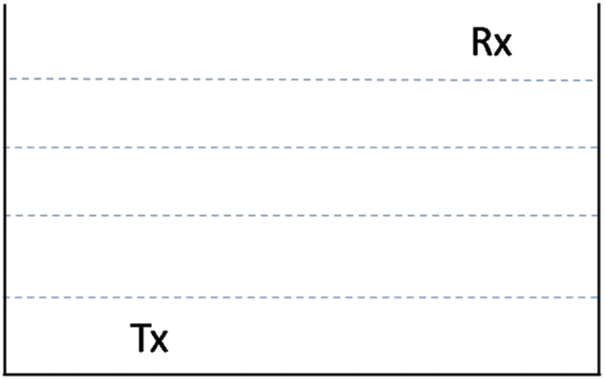
Figure 1: Illustration of ECFM implementation
Here Tx is the transmitter and is Rx the receiver in the network. It is calculated with three location points for each equipment such as (X1, X2), (Y1, Y2), and (Z1, Z2) as shown in Eq. 1
Underwater connections are made in a two-level hierarchical connection between a large number of sensors placed in the network and the BS. At the lower level, the sensors transmit data from the seabed to the sonobuoy via an optical channel. At sea level, SB collects data from sensors and sends it to the BS BS. An optical channel is created between the sensor, SB and BS BS to make these connections. During data D transfer, the data is encoded by the source node in the form of a binary B data in an array to make the data transfer with the debugging process. Fig. 2 shows the illustration of underwater network communication for a simulation environment.
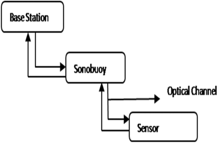
Figure 2: Illustration of a underwater network communication
When more than one piece of data travels over a network, they must first collect it and then convert it into bits as shown below.
After calculating the length of the data bits that traveled on the network, they can know how much data was transferred during that processing. Each sensor and upper-level node are equipped with a transreceiver to send and receive the packets. Pseudocode for the above operation is described below,
Bit Encoding Data Binary Conversion
Acquire D Data
Start Encode
Update Bit count
Compute Bit Count
Validate Bit Length
A transceiver that is both transmitter and receiver executed the Forward Error Correction (FEC) encoding based on the Reed-Solomon (RS) Error Detection and Correction system. Here, FEC is an error correction system that operates based on an error correction code with no response and no transmission. It is considered suitable for underwater communication as it operates without the use of a feedback redistribution system. In order to perform FEC functions properly, the transmitter connects the hamming bits HB based on the binary data to be transferred as follows.
Hamming Bits
d = data length; k = d2
n = k-1; consider 1
if (n ≤ 1); l = n + 2
else if (n ≤ 4); l = n + 3
else if (n ≤ 11); l = n + 4
else l = n + 5; update l
Hamming code is a chunk code that detects and corrects faults in two packet bit scales that arrive concurrently. These faults are a result of noise and channel defects that occur during network communication. The protocol includes a mechanism for identifying mistakes in the receiving destination of these packets, eliminating them, and then processing them. The Q-ary based RS code is calculated during the calculation using the Galois field. It is based on the unit difference with the power of 2 for the code rate and the ordered product for the error correction. RS is used to counteract the disappearance of the underwater channel. RS-FEC-codes are most suitable for the underwater channel as they have explosion errors. In addition, it is very strong and simple. Similarly, this code is in a way defined by the non-binary Galois field.
The encoded bits are modified using the corresponding modulation method. Here, Binary Phase-shift keying (BPSK), Quadrature Phase Shift Keying (QPSK), Quadrature Amplitude Modulation (QAM)16, QAM64, and QAM256 modulation methods are used to validate the encoding bits. To get the symbols according to the modulation scheme, choose Data Length (DL) and Data Bits Per Second (DBPS) as shown in Eq. 3.
Symbols are filled with padding bits. Video streaming data is transmitted from and to sensors under the sea, via an optical channel. During the transfer of data, a high-power Light Emitting Diode (LED) array is activated to perform the power multiplication process. Video processing is enabled as follows:
RS-FEC-Bit Computation Steps
Update bit count → HB
Code Length = Random(0, Bit Count)
if (i+1)2
if Hamming Code Enabled
XOR value = XOR(i+1); d = XOR Value
Store d; while d > 1
If d mod 2 = 0; Update XOR value = 0
else XOR value = 1; Update Binary Count
if(i+1)2→ 0
HB = XOR bits [Increment Binary Count]
Update HB
d = date length; k = d2
n = k-1; t = Code length
z = k – 1 – t; r = n-k
Qary HB = n, z, r
Transceiver video
Video Display → Updates Frame ID
If Video Display Count > 1
Update Frame ID = Next ID
Update Video Display
If Video Ordering Enabled
Update Count, FileName, ID, DATA, Size
Update Next ID → ID + 1
Content Stream
Update Content Stream
Save in Array [Content Stream + 1]
Array → Video Display ID
Remove Redundant ID from Array
If frame ID → Play Frame
It determines the Lambertian Angle (LA) based on the Lambertian radiation model (LRM). The optical beam reflection ratio in terms of Lambertian emission is computed between the ratio of twin natural logarithm and logarithmic cosine value of Semi-Angle (SA) at half power and it is described below, the Minimum Angle (MA) is considered as 1.
Update Sensor Counts, Check Topological Size, Packet Size
Compute LA = Angle Estimation
Update LA
while LA > Half Beam
LA- = Half Beam
cosine= cos (LA)+MA
if (( log (cos) + 1) > 0
cosine = cos (LA) + min Angle
θ = cos cosine1 m
Update θ
SA= Half Beam - LA
The LED model is calculated using the luminous intensity at an angle between the transmitter and the receiver. A half angle based on the total internal reflection is used to calculate the present confrontation of the LED. High power LED arrays can be used to create remote connection systems, such as sending and receiving data. These LEDs emit identical optical signals simultaneously. The current power of the LED is calculated as the ratio between the Flow Power (FP) and the PC. The difference between the current power and the receiving signal strength RSS signal is calculated based on the flow power distribution, here SI is the nature-meddling, and noiseless state is defined as 4.8e-9. A wideband amplifier, which is defined by intensifying the modulated signal extremely small on the protection that is peak protection is 3.1 mΩ, a flow potential FP is maximum of 29 volts, and an Extended Flow Current (EFC) maximum is 65 amps to stimulate the light-emitting diode display. For optical transmission processes, the balance of the illumination of the optical source is indispensable. It mainly linked the illumination of an LED to the number of Transmitted Currents TC as shown in Eq. (4). Further, compute the power usage during interference co-occurrence as IP. Moreover, NOP is the network region outflow power and is the Channel Capacity CC of the sensors.
Based on the optical media, the bending catalog (BAC) and Bending Angle (BA) are calculated. Refraction is the implication of various transmission channels like Air Media (AM), optical channel glass (CG), and Sea Water (SW). The Unsafe Angle (UA) of the channel is calculated using the inverse sine value of the BAC. The incidence angle of the communications is estimated as the ratio between the deflection angle and the critical angle and check event angle (EA).
BA = AM optical
else BA = optical CG
else BA SW
BAC = 1.51
If UA>0
α=EA
αa = UA
β = (360-BA)
The bending angle is calculated as the difference between the two phases with the bending angle. At this point, αa is the angle of gleaming at a bending place on the flood exterior, βa is the angle to the receiving sensor at a bending position, d1 stands for the distance between the sender and a bending position on the water area, d2 stands for the distance between a bending site and the receiving sensor, and small replication components (RC), and ρ is the bending constant. The Channel Gain (CG) of the line of vision LOV is calculated using the EA, the radiation angle, the Dist between the transceivers, the sequence of the LA, and the CG of optical saturation using the cosine function.
Non-Line Of View (NLOV) is calculated using the small reflection element coefficient, the reflection coefficient, and the cosine function and the parameters for the Line Of Sight (LOS).
In this PR is the sensor photo discovery region, line of view (LOV), and NLOV, also, the power of optical channel (OP), and power based on the distance (DP). Underwater channel loss is calculated using the beer-Lambert law, which obtains the optical power using the attenuation coefficient, connection range, the initial transmission power of the optical channel, and acquired optical power using high-speed values.
By combining the loss model with the gain of both LOV and NLOV, the total optical power obtained is calculated. Also, the quantum efficiency is computed as the ratio between the photon value (PV) and electron value (EV).
Here PV is 10e-12 and EV is 50e-9. The responsivity of the photodiode (PD) is computed using the quantum efficiency, electronic charge, wavelength of the channel, constant values. Based on the responsivity of the snow photodetector, the optical transmission power and received power are computed.
The ratio between the obtained optical power voltage and the output of the response is calculated as the slide multiplication factor and the load resistance. Calculates the RSS of channel communications using photosynthesis current, snow multiplication factor, photosynthetic noise, shady noise, and updraft noise in the optical channel.
The connection distance extension is calculated using the product of the negative constant with the attenuation value and the link range of the optical channel. On the receiver side, the optical signal is received and it is applied for the Reed-Solomon FEC process to perform the error detection and correction to obtain the decoded signal.
In the differential phase shift key modulation model, the bit signal to be sent to the encoding process is used in 5 level operations. During the modulation process, the input baseband signal is delivered to the delayed XOR as an input. Five parameters are considered in this modulation. These are: delayed - XOR, phase, delayed phase, phase difference, and base bits. In this case, if the phase difference is 0, then the existing delayed phase must be calculated. The delayed phase is the difference between the phase XORed phase and the last bit. Thus, the phase also needs to be updated. Otherwise, the phase difference can be taken as the PI value. The pseudocode for the modulation and attenuation is described below
Get attenuation
initial attenuation → 0
if(water type → pure_sea_water)
attenuation → 0.043
else if(water type → clean_ocean)
attenuation → 0.14
else if(water type → coastal)
attenuation → 0.398
else if(water type → turbid harbor)
attenuation → 2.190
Update attenuation
FEC Decoding
Update Xor value data
Update Hamming bits
if((i + 1) 2 → enabled)
if hamming code→ Enabled
xor value data = xor value data xor(i + 1)
else recvhamm ± i2 hamming–code[i]
if((xor value data × xorrecvhamm) <hbit count)
Update Receiving bit count
Return original bit → hamming bits count
Update Flipped bit (xor value data xorrecvhamm)
In the delayed XOR, the output of the XOR is given as the input of the same XOR system. The precoder, therefore, provides the output based on the previous stage signal and the current input signal. In the next step, the phase signal between the baseband signal and the delayed XOR signal is calculated as soon as the delayed XOR output is received for all input signals.
If both signals are identical then the phase signal is calculated as bit PI if it is binary-1. If both signals are identical then the phase signal is calculated as bit 0 if it is binary-0. If the baseband signal is zero and the delayed XOR signal is one then the phase signal bit is computed as PI. If the baseband signal is one and the delayed XOR signal is zero then the phase signal bit is computed as 0. Once the phase signal is calculated, the delayed phase function is activated in the next phase similar to the precoder. Here the precoder processes the signal 0 and PI instead of 0 and 1.
Once the delayed phase signal is calculated, the difference between the phase signal and the delayed signal is calculated as the phase difference. The phase difference is calculated to be similar to the calculation of the baseband and the delayed XOR. For each baseband bit, the signal value is calculated using binary encoding, and this applies to the delayed XOR bit.
The adjacent encoded signal is calculated using the Boolean XOR function based on the carrier wave signal. Now the modulated signal is calculated using the amplitude and phase modulator, which is the sum of the amplified product of the bits and the sum of the encoded signal with the inverse cosine function of the phase frequency. When retrieving the signal on the receiver side, reverse operations are performed on the modulation system to receive the first transmitted signal without signal errors. The estimation of delay and phase under delayed condition is described below,
Update delay, phase, delayed phase, phase diff, base bits
Bit length = bit counts; Initial last bit = 0
If phase difference is null
If phase→ delayed phase
If delayed phase → phase xor(phase[signal], last bit)
Delayed phase →last bit;else phase[signal] → last bit
else if phase[signal] → phase xor(delayed phase[i], last bit)
phase[signal] → last bit;else last bit → delayed phase
else delayed phase → last bit
else if phase difference → PI VALUE
if phase[signal] != delayed phase
if delayed phase → phase xor(phase[i], last bit)
delayed phase → last bit;last bit → phase[signal]
else phase[signal] → last bit
last bit → delayed phase
else if phase[signal] → phase xor(delayed phase[i], last bit)
phase[signal] → last bit;else delayed phase → last bit
last bit → phase[signal];Update bitlength
ifphase[signal] → PI VALUE
if base bits → delay XOR
if base bits → 0;base bits → 1
else No Error;else if base bits[i] → 0 && delay XOR == 1
No Error
Else if base bits[i] → 0 ;base bits[i] = 1
else if base bits[i] → 1;delay XOR[i] = 0
else if base bits →delay XOR
if base bits[i] → 0 No Error;else base bits[i] → 1
else if !base bits[i] → 0 && delay XOR[i] == 1
No Error
Else if base bits[i] → 1;Base bits[i] = 0
else if(base bits[i] → 0);delay XOR[i] = 1
last bit = 0;Update bit length
If delay XOR[i] → xor operation (base bits[i], last bit)
No Error
else if delay XOR[i] → 0;if(base bits[i] → 0)
base bits[i] → 1;
else base bits[i] → 0;else if delay XOR[i] → 0
delay XOR[i] → 1
else delay XOR[i] = 0;last bit = delay XOR[i]
Error Signal → base bits[i]
Recovered signal Update
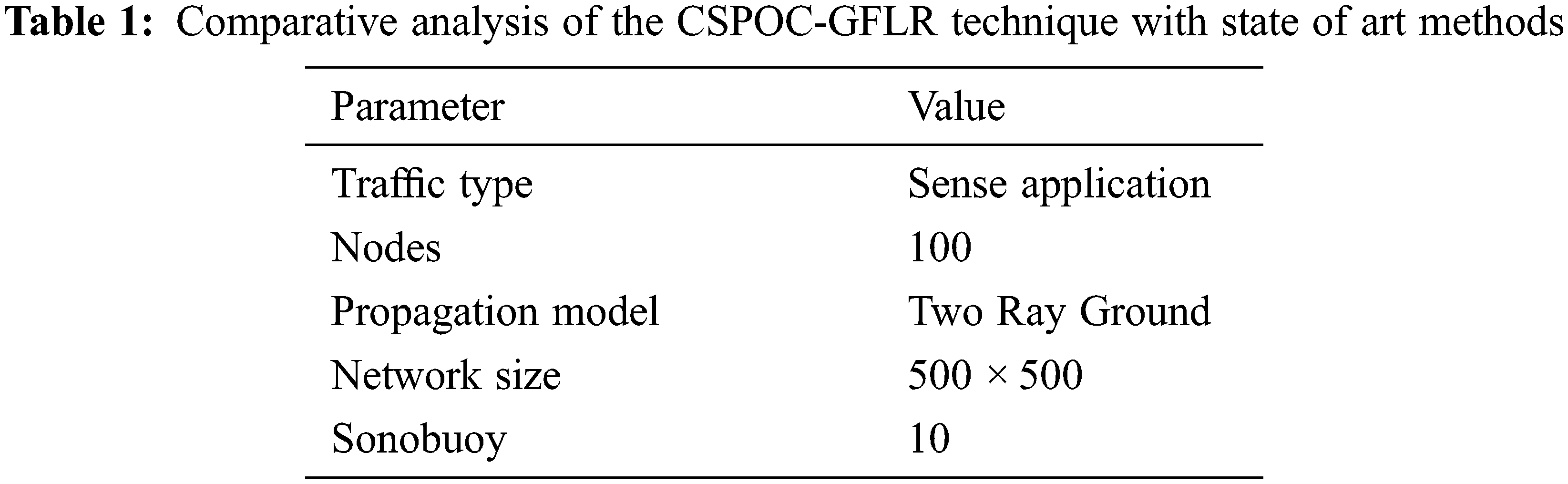
The simulation parameter used in this work is illustrated in Tab. 1. The simulated underwater optical channel model consists of 100 nodes and it has been simulated 250 times. For each simulation of configuration, the run time is assigned and the analysis of the channel model is emphasized on evaluating the performance by observing packet delivery ratio, throughput, delay, and lifetime.
The placement and communication of packet between the number of nodes, sonobuoy and base station illustrated in Fig. 3.
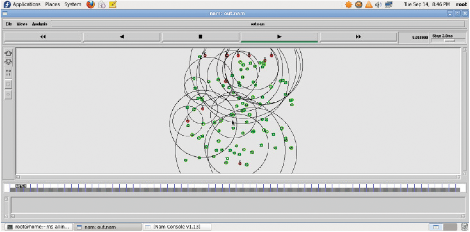
Figure 3: Transmission of data from sensor to sonobuoy and base station
During the simulation the sensor undergoes three different states such as (i) transmit (ii) receive and (iii) idle state. The amount of energy consumed by each sensor node depends on the duration it spends on each state. This can be estimated by the following equation.
where Ttxr, Trxr, and Tid denote the amount of time spent on transmitting, receive, and idle state respectively, and etxr, erxr, and eid corresponds to per-unit costs of the respective states.
Fig. 4 shows the energy profile the data packets received for every second. The result implies that the consumed energy increases with respect to the size of the packet increases in UWOC, but for the same configuration the ECFM consumes less amount of energy in the range of 345 to 380 J. So the percentage of energy-saving 25%.
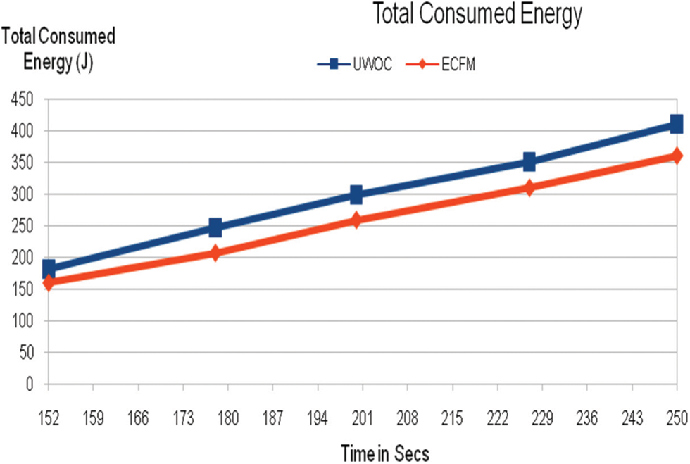
Figure 4: Simulation result of total consumed energy
Packet Delivery Ratio (PDR) can be estimated as the ratio of the total amount of data packets delivered to the total amount of data packets sent from source to destination. In general, the performance of the network can be improved when the PDR of the network increases greatly. In this paper, the performance of PDR of ECFM is compared with conventional UWOC. It observed that during the active mode, the conventional UWOC provides less PDR and moderate amount of data packets are reached to the destination node, whereas the proposed ECFM provides considerable attention on PDR and improves the performance of the network greatly as shown in Fig. 5.
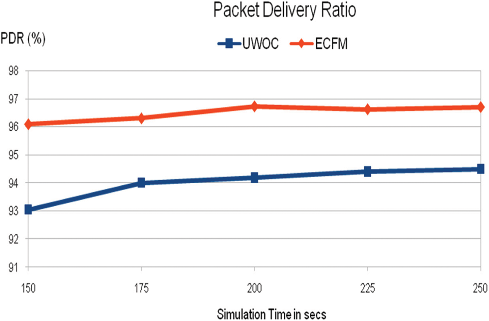
Figure 5: Simulation result of packet delivery ratio
Throughput of a network represents the amount of data packets successfully transmitted from source to destination node for unit time and it can be measured in bits per s. Simulation is performed with a packet size of 512 bytes and the network is simulated for 2 h. ECFM provides maximum throughput to 94% to 98% whereas UWOC gives 85% to 80% for the same configuration of the network as shown in Fig. 6.
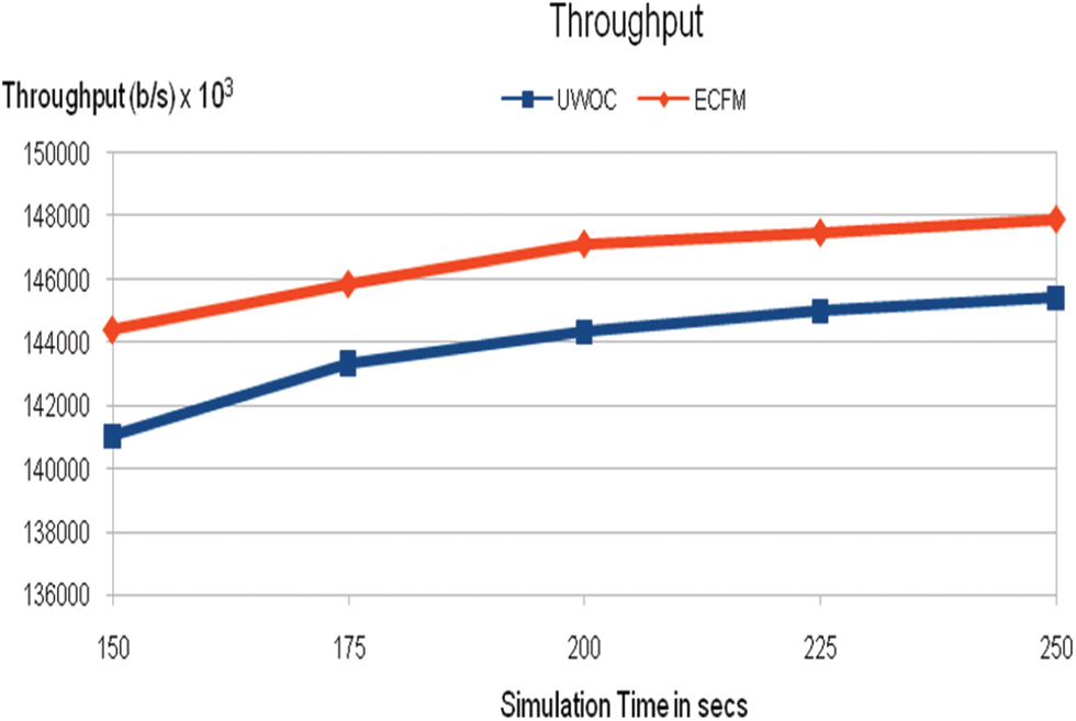
Figure 6: Simulation result of throughput
Fig. 7 illustrates the description of the number of nodes versus delay in ms of the ECFM and UWOC system. As the number of nodes in a network increases gradually the delay is reduced in ECFM than conventional UWOC architecture.
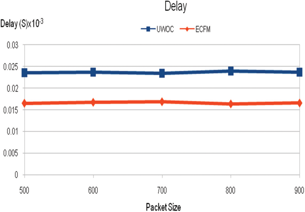
Figure 7: Simulation result of delay
To communicate with the sensors and their connection nodes, the optical channel is used. We determine the energy consumed during network connections and the energy consumed at the greatest rate when data is transferred over an optical channel. This is accomplished by selecting the photo detector to be utilised during transmission and thereby raising the strength of the receiving signal. When while data is sent and received via the same channel, the data passing through it will be somewhat different. However, due to self-interference, the data transmission distance will vary. Numerous modulation techniques enable data transport inside the water by altering the phase of the beam's wavelength carrier. We further increase the data rate by producing signals with a wide bandwidth and a short latency. Protocols will be required in the future to build a routing connection, depending on the type of the water and the contact congestion. Additionally, a void circumstance should be detected and channel selections made appropriately.
Funding Statement: The authors received no specific funding for this study.
Conflicts of Interest: The authors declare that they have no conflicts of interest to report regarding the present study.
1. R. A. Reddy, J. R. Kanth and D. Muneendra, “Under water optical wireless communication,” International Research Journal of Engineering and Technology (IRJET), vol. 5, no. 11, pp. 2395–2407, 2018. [Google Scholar]
2. J. Lloret, S. Sendra, M. Ardid and J. P. C. Rodrigues, “Underwater wireless sensor communications in the 2.4 GHz ISM frequency band,” Sensors, vol. 12, no. 4, pp. 4237–4264, 2012. [Google Scholar]
3. A. Ranjan and A. Ranjan, “Underwater wireless communication network,” Advance in Electronic and Electric Engineering, vol. 3, no. 1, pp. 41–46, 2013. [Google Scholar]
4. N. R. Krishnamoorthy and C. D. Suriyakala, “Performance of underwater acoustic channel using modified TCM OFDM coding techniques,” Indian Journal of Geo Marine Sciences, vol. 46, no. 3, pp. 117–129, 2017. [Google Scholar]
5. X. Zhang, “An investigation on large capacity transmission technologies for UWOC systems,” in Journal of Physics Conf. Series, Tianjin, China, vol. 1920, no. 12, pp. 12018–12029, 2021. [Google Scholar]
6. L. Liu, S. Zhou and J. H. Cui, “Prospects and problems of wireless communication for underwater sensor networks,” Wireless Communications and Mobile Computing, vol. 8, pp. 977–994, 2008. [Google Scholar]
7. B. Renner, J. Heitmann and F. Steinmetz, “AHOI: Inexpensive, low-power communication and localization for underwater sensor networks and μAUVs,” ACM Transactions on Sensor Networks, vol. 16, no. 12, pp. 1–46, 2020. [Google Scholar]
8. S. Fattah, A. Gani, I. Ahmedy, M. Y. I. Idris and I. A. Hashem, “A survey on underwater wireless sensor networks: Requirements, taxonomy, recent advances, and open research challenges,” Sensors, vol. 20, no. 18, pp. 5381–5393, 2020. [Google Scholar]
9. B. Pranitha and L. Anjaneyulu, “Analysis of equalization acoustic communication system using equalization technique for ISI reduction,” in Int. Conf. on Computational Intelligence and Data Science (ICCIDS), Warangal, India, vol. 1, no. 167, pp. 1128–1138, 2019. [Google Scholar]
10. K. Chithra, N. Sireesha, C. Thangavel, V. Gowthaman, S. S. Narayanan et al., “Underwater communication implementation with OFDM,” Indian Journal of Geo-Marine Sciences, vol. 44, no. 2, pp. 259–266, 2014. [Google Scholar]
11. N. Saeed, A. Celik, Y. A. Naffouri and M. Alouini, “Underwater optical wireless communications, networking, and localization: A survey,” Ad Hoc Networks, vol. 1, no. 94, pp. 174–192, 2018. [Google Scholar]
12. D. Anguita, D. Brizzolara and G. Parodi, “Building an underwater wireless sensor network based on optical communication: Research challenges and current results,” in 3rd Int. Conf. on Sensor Technologies and Applications, Athens, Greece, vol. 9, no. 5, pp. 476–479, 2009. [Google Scholar]
13. X. Wu, W. Xue and X. Shu, “Design and implementation of underwater wireless electromagnetic communication system,” in AIP Conf. Proc. Green Energy and Sustainable Development, Boca Raton, Florida, vol. 1864, no.1, pp. 2024–2035, 2017. [Google Scholar]
14. S. Ryecroft, A. Shaw, P. Fergus, P. Kot, K. Hashim et al., “A first implementation of underwater communications in raw water using the 433 MHz frequency combined with a bowtie antenna,” Sensors, vol. 19, no. 8, pp. 1813–1825, 2019. [Google Scholar]
15. P. Ranjitharajan, P. T. Elizabeth, A. Susan Roy, K. S. Aiswarya and A. Christymolbousally, “Underwater wireless communication system,” International Journal of Engineering Research & Technology (IJERT), vol. 9, no. 12, pp. 121–134, 2020. [Google Scholar]
16. M. F. Ali, D. Nalin, K. Jayakody and S. Dmitry, “Recent advances and future directions on underwater wireless communications,” Archives of Computational Methods in Engineering, vol. 27, no. 5, pp. 1397–1412, 2019. [Google Scholar]
17. S. A. Hassnainmohsan, M. M. Hasan, A. Mazinani, M. A. Sadiq, M. H. Akhtar et al., “A systematic review on practical considerations, recent advances and research challenges in underwater optical wireless communication,” International Journal of Advanced Computer Science and Applications(IJACSA), vol. 11, no. 7, pp. 11–17, 2020. [Google Scholar]
18. G. Iandra and L. R. Marcello, “Performance evaluation of multicarrier systems applied to underwater acoustic communications,” Electronics, vol. 16, no. 41, pp. 2166–9589, 2020. [Google Scholar]
19. D. Menaka, C. Sabithagauni, T. Manimegalai and K. Kalimuthu, “Design of low power hybrid communication model,” Wireless Personal Communications, vol. 12, no. 5, pp. 331–345, 2021. [Google Scholar]
20. R. B. Ruiz, P. S. Serrano, P. C. Vázquez, B. G. Zambrana and J. M. G. Balsells, “Capacity of underwater optical wireless communication systems over salinity-induced oceanic turbulence channels with ISI,” Optics Express, vol. 29, no. 15, pp. 23142–23158, 2021. [Google Scholar]
21. F. Ian, F. Akyildiz, D. Pompili and T. Melodia, “Challenges for efficient communication in underwater acoustic sensor networks,” ACM Sigbed Review, vol. 1, no. 2, pp. 3–8, 2004. [Google Scholar]
22. K. Hemanikaushal and G. Kaddoum, “Underwater optical wireless communication,” IEEE Access, vol. 4, no. 6, pp. 1518–1547, 2016. [Google Scholar]
23. J. Liu, J. Wang, S. Song, J. Cui, X. Wang et al., “MMNET: A multi-modal network architecture for underwater networking,” Electronics, vol. 9, no. 12, pp. 2184–2196, 2020. [Google Scholar]
 | This work is licensed under a Creative Commons Attribution 4.0 International License, which permits unrestricted use, distribution, and reproduction in any medium, provided the original work is properly cited. |