DOI:10.32604/iasc.2022.025792
| Intelligent Automation & Soft Computing DOI:10.32604/iasc.2022.025792 | |
| Article |
IoT Based Disease Prediction Using Mapreduce and LSQN3 Techniques
1Department of Computer Science and Engineering, Dhanalakshmi Srinivasan Engineering College, Perambalur, 621212, India
2Department of Computer Science and Engineering, SRM Institute of Science and Technology, Ramapuram, 600089, India
3Directorate of Distance Education, Alagappa University, Karaikudi, 630003, India
4Department of Electrical and Electronics Engineering, Sathyabama Institute of Science and Technology, Chennai, 600119, India
5Department of Information Technology, Sona College of Technology, Salem, 636005, India
6Department of Computer Science and Engineering, VNR Vignana Jyothi Institute of Engineering and Technology, Hyderabad, 500090, India
7Department of Computer Science, KIET Group of Institutions, Delhi NCR, Ghaziabad, 201206, India
*Corresponding Author: R. Gopi. Email: gopircse@gmail.com
Received: 05 December 2021; Accepted: 19 January 2022
Abstract: In this modern era, the transformation of conventional objects into smart ones via internet vitality, data management, together with many more are the main aim of the Internet of Things (IoT) centered Big Data (BD) analysis. In the past few years, significant augmentation in the IoT-centered Healthcare (HC) monitoring can be seen. Nevertheless, the merging of health-specific parameters along with IoT-centric Health Monitoring (HM) systems with BD handling ability is turned out to be a complicated research scope. With the aid of Map-Reduce and LSQN3 techniques, this paper proposed IoT devices in Wireless Sensors Networks (WSN) centered BD Mining (BDM) approach. Initially, the heart disease prediction dataset is acquired from publicly available sources in the proposed approach. Following that, the dataset is mitigated by reducing redundant data using Map-Reduce and making it useful for the upcoming examination. During the mapping step, the Linear Log induced K-Means Algorithm (LL-KMA) clustering algorithm is used. The LF-CSO technique is used in the reduction phase to select the optimal Cluster Centroids (CC). The features are extracted from the reduced data. After that, utilizing the Pearson Correlation Coefficient based Generalized Discriminant Analysis (PCC-GDA), the extracted features’ dimensionality is mitigated. Subsequently, the features being reduced are neumaralised for classification purposes. Lastly, to classify the disease, the Log Sigmoid activation based Quasi-Newton Neural network (LSQN3) classifier is employed. The proposed method is contrasted with the existing methodologies to assess the performance. The experiential outcomes displayed that the proposed work is highly efficient than the other methodologies.
Keywords: Big data mining; mapreduce; k-means algorithm; disease prediction system; real-time health monitoring; cat swarm optimization (CSO); feature reduction
Recently, there has been an increase in the total number of patients suffering from chronic diseases, Hypertension and other health issues as a result of unhealthy dietary habits, human emotions, lack of physical activity, alcohol consumption, surrounding environmental conditions and other unhealthy practices [1,2]. As a result, in order to avert fatal situations, individuals’ health status must be observed and examined in their daily lives [3]. Furthermore, the patient must learn monitoring knowledge related to their health condition, which helps healthy life care routines [4]. The use of wireless HM for chronically ill patients and the elderly improves the quality of life [5]. Unnecessary hospitalizations could be avoided by using remote HM, lowering healthcare costs while improving care quality [6]. This tailored HC system with IoT application efficiently benefits personal health [7]. IoT, a primary technology, connects every object in daily life, including sensors, devices and systems. Many WSNs are covered by IoT-centered HC networks [8]. This WSN is used in a patient for continuous monitoring of health issues. WSN detects physiological signals such as electrocardiogram (ECG), blood oxygen (SpO2), blood pressure (BP), blood glucose and user actions such as sitting, standing, walking and so on [9]. These monitoring parameters are used in automated decision support systems. It could help doctors make an early diagnosis [10].
Human health parameters often follow a regular behaviour. Patients would encounter imbalance circumstances of health indicators such as high temperature, low blood pressure and so on when they suffer from chronic disease [11,12]. Thus, in terms of health-related parameter management and analysis, analyzing such regular behaviour information as of the acquired data facilitates the investigation of new characteristics [13]. However, the widespread use of IoT-based HC systems generates a massive amount of medical data [14]. Examining such BD for better decision-making is a complicated and time-consuming endeavors [15].
To address this, many existing algorithms as well as Machine Learning (ML) methodologies are described. Despite deep learning’s immense capacity for managing massive amounts of data [16,17], learning models require a large amount of memory and a significant compute cost. ML models were quite efficient in a variety of domains. However, due to latency limits, ML has only had a limited applicability in clinical decision support systems [18]. Despite the fact that health behaviours are predicted and tracked using existing methodologies [19,20], the prediction rate and early prediction procedure are still insufficient. Thus, the paper proposes IoT devices in a WSN-based Disease Prediction System (DPS) with BDM using Map-Reduce and LSQN3 algorithms.
This paper is classified as follows: Section 2 examines the related works in relation to the suggested technique. Section 3 describes the planned study titled IoT devices in WSN-based DPS with BDM using Map-Reduce and LSQN3 algorithms. Section 4 displays the findings and discussion for the suggested work, which is centred on performance indicators. Finally, Section 5 provides a conclusion with recommendations for further work.
Bharathi et al. [21] developed an Energy Efficient Particle Swarms Optimization centred Clustering-Artificial neural network (EEPSOC-ANN) that achieved energy clustering as well as disease diagnostics through IoT devices. The ‘three’ key subsystems in which the designed model functioned were the user subsystem, the cloud subsystem and the alert subsystem. The original user subsystem involved in data collecting was taken care of by IoT medical devices as the user. Concurrently, the EEPSOC was carried out. The IoT devices were clustered and the Cluster Head (CH) was properly picked. The detected data from IoT devices was then sent to gateway devices and the cloud subsystem. Finally, ANN performed disease diagnosis on the cloud subsystem. The sickness was accurately anticipated with varying degrees of severity and an alarm system was set up. Effective performance was indicated by an average maximum sensitivity (96.094%), specificity (93.492%), accuracy (94.066%) and F-score value (94.066%). The EEPSOC-ANN was both an energy-efficient and effective diagnosis model. Nonetheless, the scheme was inept when it came to unstructured data.
Sood et al. [22] developed an IoT-Fog-based HC system for continuous monitoring and analysis of blood pressure statistics in order to foresee hypertensive patients. The hypertension stage was initially identified based on the user’s health data. The fog layer was where the IoT sensors were collected. Following hypertensive stage recognition, the ANN was used to forecast the risk level of hypertension attacks in users at remote sites. An important feature of the technology was the continuous generation of emergency notifications of BP variation as of fog systems to hypertensive users on their phones. The temporal information created as a result of the fog layer was used to provide preventive actions as well as timely recommendations for patients’ wellness. The created framework achieved lower response time, improved accuracy and bandwidth efficiency. The system, however, had the limitation of improper feature selection.
Pathinarupothi et al. [23] designed an IoT-centered smart edge architecture for remote HM, in which wearable imperative sensors relayed data to the IoT smart edge. Rapid Acting Substances The ‘2’ higher-performance software engine summarized for effective PROgnosis (RASPRO) as well as Criticality Measure Index (CMI). Both software engines were active on the IoT smart edge. The RASPRO turned the extensive sensor data into clinically relevant summaries on the Personalized Health Motif (PHM) as well as warnings. The PHM and alarms were then delivered to the physicians using the best combination of cellular or mobile or NB-IoT networks based on a risk-stratified push or pull protocol. The approach achieved precision (0.87), recall (0.83) and F1-score (0.85). Significant reductions in bandwidth (98%) and energy (90%) were seen. The method was suitable for narrow-band IoT networks. The technique, however, was confined to higher-dimensional inputting data.
Ismail et al. [24] proposed a CNN-based health model for normal health factor analysis in the medical IoT environment. The health conditions and lifestyle habits associated with chronic diseases were gathered using IoT devices. The double-layer fully connected CNN structure was then used to classify the acquired data. The most important health-related indicators were chosen for the ‘first’ Hidden Layer (HL). In the second layer, a correlation co-efficient analysis was performed with the goal of classifying both positively and negatively connected health aspects. Regular patterns’ activities were discovered by mining the usual pattern recurrence among the defined health parameters. The model’s output was subdivided into regular-correlated factors associated with obesity, high blood pressure and diabetes. The CNN-regular knowledge discovery model’s efforts were minimised by the use of ‘2’ separate datasets. Better accuracy and lesser computing load were realised. However, the scheme had an over-fitting problem.
Ravichandran [25] proposed an IoT-based health monitoring system. The designed solution for continuous wireless patient monitoring included a mobile application as well as GSM. The main contribution was the development of a dependable patient management system based on IoT. As a result, HC experts used an IoT-centered integrated HC system to monitor patients and ensure quality patient care. The fundamental parameters were tracked by the sensors. The collected data was then transmitted to the cloud via a Wi-Fi module. It was developed a wireless HC monitoring system. Real-time online information on the patient’s circumstances, such as temperature, ECG, heartbeat rate, BP rate and so on, was made available. This data was sent to the doctor’s mobile device, which included the programme. If any of the parameters exceeded the threshold value, an alert message was sent to the doctor’s phone. The other top-tier approaches were thrashed. There were limitations, such as significant computing overhead and large memory requirements.
3 Equations and Mathematical Expressions
WSN is now an important component of hospital HC monitoring systems. In emergency scenarios, it provides medical monitoring, memory augmentation, and contact with the HC provider. With the continuous HM with implantable and wearable devices, the correct detection capabilities of emergency circumstances for at-risk patients would be improved. To provide prompt treatment, the HC monitoring system can quickly understand individuals with varying degrees of attention as well as physical limitations. Wearable medical equipment equipped with sensors create massive amounts of data on a continuous basis. BD is a common abbreviation for it. Because of the complexities of the data, it is difficult to process and analyse the BD in order to identify meaningful information that can be used in decision making. As a result, BD analytical techniques are required for the storage, processing, and analysis of large amounts of data. The BD analytics in HC provides insight into very huge datasets. It also helps to improve outcomes while keeping expenses down. As a result, this work presents a WSN-centered BDM approach for creating illness prediction mechanisms using Map-Reduce and LSQN3 techniques. The ‘6’ processes employed here to train the system are data collection, Map-Reduce, feature extraction (FE), feature reduction (FR), numeralization, and classification. The sensed patient health data is considered when testing the system. Fig. 1 shows the block diagram for the suggested model.

Figure 1: Block diagram of the proposed model
For training the system, data from publicly available heart disease prediction sources, such as the UCI hub, is used. The collected data includes IoT-sensed patient health information. The Map-Reduce approach is used to reduce the size of a dataset due to its massive amount of data. Initially, the dataset’s data quantity is described as,
Wherein, i = 1, 2, …, n signifies the number of data present primarily.
Map-Reduce distributes a big amount of data as smaller portions of clusters through the data distribution. It is essentially a programming model. The ‘2’ steps are the Map and Reduce functions. The inputted dataset is divided into smaller subunits, and the data is then processed in parallel in key or value pairs form. This process is handled by the map function. The mapped data is then sorted and transmitted to the reduced function. This function abridges repetitive data and hence returns a single output value. The optimum cluster centres are then selected. Clustering is repeated to improve accuracy. In the mapping phase, the LL-KMA is used to cluster the data; in the reducer phase, the Levy Flight amalgamated Cat Swarm Optimization (LS-CSO) is used. The Map-Reduce function process is described in further detail.
At first, the data (xi) is amassed in the Map-Reduce system’s storage unit and is inputted to the mapper. To reduce the amount of the data load, the data is divided into smaller chunks and shared across mappers. The LL-KMA is used to reduce the amount of data exchanged. It categorizes the data into similar clusters. The mapping function will be finished completely prior to the reduction step. The K-Means Algorithm (KMA) groups data by first assigning the total number of clusters, which is a clustering approach. The centroid locations for grouping the clusters are created at random and are centred on the entire number of clusters. The data points are then transferred to the nearby cluster centre based on the Euclidean distance. Because of the arbitrary production of CC, the system’s processing time increases. It also includes the possibility of getting unfavourable results. The objective function of a common KMA is split using a linear log weight function to improve the system’s effectiveness. As a result of this improvement, better clustering performance can be obtained, as well as a reduction in processing time. Liners Log (LL) adapted KMA is the name given to this adaptation to the KMA (LL-KMA).
The LL-KMA steps are elucidated below.
Let, (Ck = C1, C2, …, CK) be the arbitrarily chosen initial CC of the inputted data (xi). The Euclidean distance (Ed) betwixt the cluster centroids (Ck) and the data point (xi) is gauged as,
The data points are assigned based on their proximity to the nearest cluster centres using the shortest distance measurements.
The linear log weighted objective function (ξ) is gauged utilizing Eq. (3),
Wherein, L(w) signifies the linear log weight function and is rendered as,
The process continues via varying the CC. The iteration continues until the CC is not changed. Lastly, the clustered group of data (yj) is attained, which is denoted as,
Here, N signifies the number of clustered groups.
This is the last phase of the Map-Reduce system. The execution phase begins only when the mapping step is completed. The reducer function sorts the mapper-generated cluster and calculates the viable CC. The data is then grouped again using these centroid points. It just included the reduced data. The LF-CSO technique was used to construct the feasible CC in this case. Cat Swarm Optimization (CSO) was created to demonstrate the natural behaviour of cats. It was based on the swarm optimization method. It was discovered that cats spend little time seeking for prey and spend the majority of their time relaxing and observing their surroundings. The ‘2’ modes included in this are seeking mode and tracing mode. Each cat includes their position, velocity, and Fitness Value (FV) for each dimension. Cats constantly gaze about in searching mode to find the target prey. In tracking mode, it walks softly step by step until it discovers and grabs the target. However, due to the large memory expenditure of the CSO limitations, its convergence speed and optimization accuracy are constrained. As a result, the random value generated during the cat’s velocity updating phase is adjusted with the Levy Flight (LF) distribution to improve convergence speed and accuracy. LF calculates the arbitrary number based on the cat’s arbitrary steps and jumps as determined by step length. As a result, the LF-induced CSO is referred to as LF-CSO, as explained further below
Step 1: Let the initial populace of cats be yj = y1, y2, …, yN and
Step 2: Subsequently, the fitness of every cat
1) Seeking mode
In this mode, the cat is at rest and detects prey or a threat in its surroundings. If any prey or danger is spotted, it begins to move slowly and carefully. It is identified as the local search for a solution. This mode includes the following basic components: Seeking Memory Pool (SMP), Dimension Change Count (DCC), Seeking Range of Selected Dimension (SRSD), Self-Position Consideration (SPC), and Mixture Ratio (MR).
a) SMP defines the number of copies made by every cat in the seeking process.
b) SRSD mentions the difference betwixt the old and new dimensions of the cat chosen for mutation.
c) DCC determines the total dimensions a cat position undergoes for mutation.
d) SPC is basically the Boolean variable that signifies the cat’s current position as a candidate position for movement.
e) MR defines that most of the time the cats spend taking rest as well as observing.
Step 3: Generate m copies of every cat (yj). If the cat’s current position is equivalent to the candidate position, then m − 1 copies of cat are made and the cat’s current position remains as one of the copies.
Step 4: For every copy of a cat m, a new position
In Eq. (6), ψ signifies the difference between the old and new dimension of cat,
Step 5: Next, the fitness of the new position
Wherein,
2) Tracing mode
Step 6: The cat decides its movement speed and direction after finding a prey while resting, based on the position and speed of the prey. The cat’s velocity in D−dimensional solution space is expressed as,
Here, κ signifies a constant and ℓ implies the levy flight distribution and is gauged utilizing Eq. (9),
In the above-given equation, γ, o signifies the normal distribution function and
Wherein, χ signifies the standard gamma function.
Step 7: The cat with this velocity moves in the D−dimensional solution space and then reports every position it takes. The cat velocity is set to maximum velocity if it is above the maximum velocity. The new position of each cat
In (11),
Step 8: The cats are then re-picked by computing the FV for the new cat position and putting them in tracing and searching mode centred on MR. The process will be repeated until a better option is found. A better solution elucidates the optimum CC. The data is then clustered again to obtain accurate clusters centred on these centroids. Subsequent to re-clustering, the last output of the reducer becomes the reduced dataset (R(j)) that encompasses M-amount of data.
The LF-CSO’s pseudocode is shown in Fig. 2.

Figure 2: Pseudocode of the proposed LF-CSO technique
Next, the features are extracted for additional analysis as of the reduced data (R(j)). Age, sex, chest pain type, resting BP, serum cholesterol, fasting BP, etc. are some features that were extracted. The process of extracting the necessary information as of the dataset is the FE, which is employed for classification. The Knumber of extracted features (f(k)) is rendered below,
3.4 Feature Reduction by Means of PCC-GDA
Following FE, FR is performed, which maps the higher-dimensional features on the lower-dimensional subspace without losing discriminant information. The features of the proposed work were minimised by PCC-GDA. The Generalized Discriminants Analysis (GDA) technique is essentially a non-linear FR technique. The goal is to find a projection matrix for features on a low-dimensional space by maximizing the ratio between the between-class scatter matrix and the within-class scatter matrix. If the information is not available in the computed class, the dimensionality reduction results are erroneous. To maintain the system’s correctness, the Pearson Correlations Coefficient (PCC) is used to gauge the between-class scatter matrix, which uses the mean class values for computation. This GDA correction is known as PCC-GDA. PCC-GDA is depicted as,
First, PCC-GDA maps the feature vector f in space F to reduced feature vectors η(f(k)) in space X. Consider K be the number of classes in the class (f(k)) and the between-class scatter matrix s(b) is computed utilizing Eq. (14),
In the above-given equation, μk and
The with-in class scatter matrix s(w) is estimated below,
Subsequent to the scattering matrix calculation, the kernel function (k(fp, fq)) is formulated as
Here, p, q range from 1 ≤ p, q ≤ K.
The solution is attained by means of solving the Eq. (17),
Wherein, β signifies the co-efficient vector, K implies the kernel matrix and D implies the block diagonal matrix. β satisfies the condition,
Wherein,
The kernel matrix K is gauged utilizing the subsequent equation,
Wherein, A implies the Eigen vector matrix and
Thus, by means of solving Eq. (17), the dimensionality reduced feature is attained. The set of reduced features (r(i)) are shown as,
In (20), N signifies the number of features in the reduced dataset. Next, the numeralization technique occurs.
The symbolic aspects of the data must be converted into numerical features in order for the data to be useful for further analysis. The categorical attributes’ values are replaced with numeric values. This is accomplished by mapping any integer value between 1 and different values based on the data type. At the completion of this procedure, all of the information is converted into numbers, which are then used for classification.
The numeralized features
These normalised features are then fed into the classifier, which uses them to differentiate between diseased and non-diseased data.
3.6 Classification by Means of LSQN3
The neural network (NN) is used for categorization in this case. It consists of the Input Layer (IL), the Hierarchical Layer (HL), and the Output Layer (OL). To begin, the numeralized data is sent to the NN’s IL. The data is then passed to the HL by the IL. In the HL, random weight values are generated. The neurons in each HL were stimulated by the Activation Function (AF). As a result, the generic AF utilised in the NN may slow down the classification process. It resulted in a longer training period as well as a decrease in system accuracy. As a result, the Log Sigmoid (LS) AF replaces the network’s general AF. Furthermore, the Quasi-Newton (QN) technique is used to minimise the NN’s loss function. It is the so-called LSQN3 because of these modifications in the traditional NN. The LSQN3 is detailed below and the general NN architecture is cited in Fig. 3.

Figure 3: General architecture of NN
Step 1: Firstly, the numeralized features
Wherein, B(jH) signifies the bias value in every node (j) of the HL.
Step 2: The LS activation function (δ(H(j))) of the HL can well be computed as,
Step 3: Next, the output layer (O(j)) can be well described by,
Wherein, B(jO) signifies the output layer bias value and W(H−O) implies the hidden-output weight value.
Step 4: The error value (err) is gauged by Eq. (25),
In Eq. (25), T(i) implies the targeted output and Y(i) signifies the obtained output of the NN classifier. In the proposed NN, the error function is minimized by means of the Quasi-Newton (QN) method intended for the weight updating process.
Step 5: The error function (err) is minimized utilizing the below QN equation,
Here, m = 0, 1, 2, …M signifies the iteration count, Tm implies the training rate and Hm, hm signifies the inverse Hessian approximation. For reducing the error function, error minimization is employed in the training process. The NN utilizes the updated weights for better classification in the testing time. Lastly, the diseased data and non-diseased data are classified by the classifier.
Patient registration occurs first during the testing phase. Following successful registration, patients are prompted to log in. Following that, data from the patients’ wearable devices is sensed and stored in the hospital cloud server. During doctor login, the patient IoT data is downloaded to the doctor’s system. Following that, operations such as FE, FR, numeralization, and categorization continue. Finally, the classifier determines whether or not it is a disease based on the observed symptoms.
This section explains in detail the end result of the proposed method. The proposed work’s efficiency is determined through performance and comparison analysis. The suggested project is written in JAVA. The data are taken from the Heart disease UCI dataset, which is publicly available on the Internet.
4.1 Performance Analysis of Proposed Clustering Technique (LL-KMA)
The suggested LL-KMA clustering algorithm’s performance is validated using clustering time and clustering accuracy. Following that, the proposed approach is analogized using numerous current techniques, including K-means, Fuzzy C-Means (FCM), K-Medoid and Mean shift, to demonstrate its utility. The suggested LL-KMA clustering algorithm’s performance is validated using clustering time and clustering accuracy. Following that, the proposed approach is analogized using numerous current techniques, including K-means, Fuzzy C-Means (FCM), K-Medoid and Mean shift, to demonstrate its utility.
Tab. 1 shows the clustering time achieved by the proposed LL-KMA clustering algorithm as well as the other clustering techniques K-Means, FCM, K-Medoid and Mean shift. According to a comparison study, the LL-KMA algorithm forms the effective cluster in a limited duration of 21367 ms. However, the available clustering techniques, notably K-means, FCM, K-Medoid and Mean shift, require 22958, 26537, 30218 and 33821 ms to construct an efficient cluster. As a result, the augmenting time for cluster formation may have an effect on the entire execution time of the operation. Among the existing clustering approaches, the LL-KMA completes the clustering process quickly. As a result, the overall performance of the suggested task could be improved.

Fig. 4 compares the clustering accuracy of the proposed LL-KMA to the existing works, notably K-means, FCM, K-Medoid and Mean shift. According to the comparison study, the proposed work forms a cluster with a high accuracy rate of 96%, while the clustering accuracy of the prevalent clustering algorithms, namely K-means, FCM, K-Medoid and Mean shift, is 87%, 83%, 75% and 71%, respectively. When compared to the proposed work, this is literally less. Thus, when compared to existing methods, the LL-KMA exhibits notable performance in cluster creation. Furthermore, this precise cluster formation has a greater impact on categorization accuracy.

Figure 4: Comparative analysis of the proposed LL-KMA in terms of clustering accuracy
4.2 Performance Analysis of Proposed Optimization Algorithm (LF-CSO)
The performance of the LF-CSO optimization algorithm is evaluated based on fitness vs. iteration. To demonstrate the value of the proposed work, it is compared to known algorithms such as Cat Swarm Optimization (CSO), Harris Hawks Optimization (HHO), Whale Optimization Algorithm (WOA) and Particle Swarm Optimization (PSO).
Fig. 5 compares the proposed LF-CSO to existing algorithms such as CSO, HHO, WOA and PSO. Essentially, the fitness vs. iteration hypothesis asserts that the approach achieves the best FV in the fewest iterations, allowing the computing time to be greatly reduced. According to that, the LF-CSO provides the best answer with the fewest iterations. The existing solutions, however, require more iteration to offer the best result. As a result, when compared to the suggested LF-CSO, the overall execution time of the existing models is longer. As a result, the LF-CSO achieves the best FVs. The best option is supplied as soon as feasible and the offered one ensures classification accuracy.

Figure 5: Comparative analysis of the proposed LF-CSO with respect to fitness vs. iteration
4.3 Performance Analysis of Proposed Classification (LSQN3)
To determine the model’s significance, the proposed LSQN3 is evaluated using various performance metrics such as accuracy, sensitivity, specificity, precision, recall, F-measure, False positive rate (FPR), False Negative rate (FNR) and Matthew’s correlation coefficient (MCC) and compared to previous works such as Decision tree, Nave Bayes, Support vector machine and K-Nearest Neighbour.
Tab. 2 includes the value of performance metrics such as specificity, sensitivity, and accuracy of the LSQN3 and other existing works such as Decision tree, Nave Bayes, SVM, and KNN. Tabulation 2 clearly shows that the proposed one achieves 96.15 percent accuracy, 96.21 percent sensitivity, and 95.67 percent specificity. However, existing methodologies achieve accuracy of 91.26 percent on average, sensitivity of 91.69 percent on average, and specificity of 89.67 percent on average. As a result, the LSQN3 achieves high-performance metrics and the suggested effort accurately examines huge data and more precisely monitors patient health condition.

Tab. 1 is depicted graphically in Fig. 6. In this case, the LSQN3’s accuracy, sensitivity, and specificity are compared against existing algorithms such as Decision tree, Nave Bayes, SVM, and KNN. The model’s effectiveness is determined by its accuracy, sensitivity, and specificity rates. Based on the total comparison, it is clear that the proposed one has a greater rate of performance measures. This increased metrics rate demonstrates the suggested model’s significant efficiency. Furthermore, the suggested work is critical to the healthcare monitoring system.

Figure 6: Graphical representation of the proposed LSQN3 based on accuracy, sensitivity and specificity
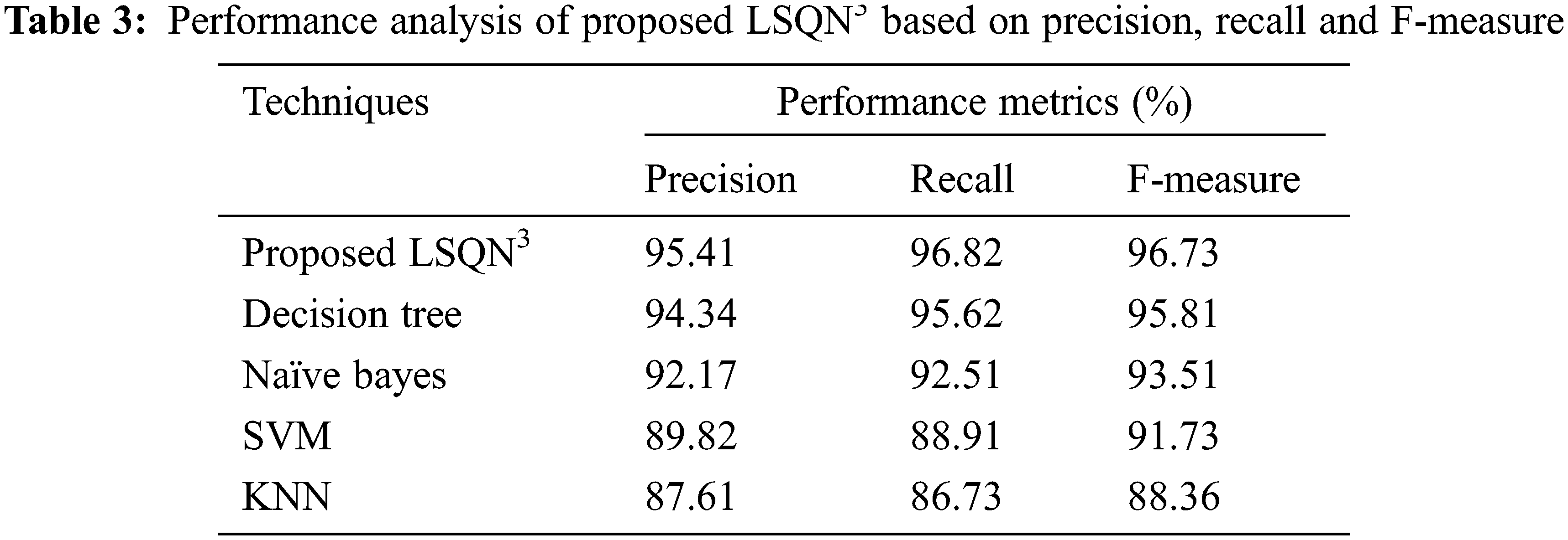
In terms of precision, recall, and F-measure, the performance analysis of the proposed LSQN3 with several existing approaches is shown in Tab. 3. According to the data, the proposed method achieves 95.41% precision, 96.82% recall, and 96.73% F-measure, whereas the existing methods achieve precision rates ranging from 87.61% to 94.34%, recall rates ranging from 86.73% to 95.62%, and F-measure rates ranging from 88.36 percent to 95.81%. As a result, the proposed one in the IoT healthcare monitoring system effectively handles unknown circumstances and achieves superior results.
The paper presented IoT devices in WSN-centered DPS with BDM using Map-Reduce and LSQN3 algorithms. The suggested framework includes numerous operations such as HC-IoT data collecting, map reducing function, FE, FR, Numeralization and Classification. Following that, the experimentation analysis is carried out. To validate the suggested algorithm’s effectiveness, the performance of the proposed methodologies is analysed, as well as a comparison examination of key performance measures. Diverse uncertainties may be handled by the developed approach, which also yields more favourable outcomes. The publicly available Heart disease UCI dataset is used in the analysis. The proposed technique achieves 96.15% accuracy, 96.21% sensitivity and 95.67% specificity. Furthermore, the suggested clustering technique achieves an effective cluster in a limited period, say 21367 ms, with a 96% accuracy rate. The suggested illness prediction framework easily outperforms the best approaches. In the future, the work will be expanded with some sophisticated NN and the DPS will be performed on more challenging datasets.
Funding Statement: The authors received no specific funding for this study.
Conflicts of Interest: The authors declare that they have no conflicts of interest to report regarding the present study.
1. H. Ren, H. Jin, C. Chen, H. Ghayvat and W. Chen, “A novel cardiac auscultation monitoring system based on wireless sensing for healthcare,” IEEE Journal of Translational Engineering in Health and Medicine, vol. 6, pp. 1–12, 2018. [Google Scholar]
2. C. Yi and J. Cai, “A truthful mechanism for scheduling delay-constrained wireless transmissions in IoT-based healthcare networks,” IEEE Transactions on Wireless Communications, vol. 18, no. 2, pp. 912–925, 2018. [Google Scholar]
3. K. N. Qureshi, S. Din, G. Jeon and F. Piccialli, “An accurate and dynamic predictive model for a smart M-health system using machine learning,” Information Sciences, vol. 538, pp. 486–502, 2020. [Google Scholar]
4. P. Gope and T. Hwang, “BSN-care: A secure IoT-based modern healthcare system using body sensor network,” IEEE Sensors Journal, vol. 16, no. 5, pp. 1368–1376, 2015. [Google Scholar]
5. W. Huifeng, S. N. Kadry and E. D. Raj, “Continuous health monitoring of sportsperson using IoT devices based wearable technology,” Computer Communications, vol. 160, pp. 588–595, 2020. [Google Scholar]
6. C. Pretty Diana Cyril, J. Rene Beulah, N. Subramani, P. Mohan, A. Harshavardhan et al., “An automated learning model for sentiment analysis and data classification of twitter data using balanced CA-SVM,” Concurrent Engineering: Research and Applications, vol. 29, no. 4, pp. 386–395, 2021. [Google Scholar]
7. N. Dey, A. S. Ashour, F. Shi, S. J. Fong and R. S. Sherratt, “Developing residential wireless sensor networks for ECG healthcare monitoring,” IEEE Transactions on Consumer Electronics, vol. 63, no. 4, pp. 442–449, 2017. [Google Scholar]
8. M. A. Berlin, S. Tripathi, V. Brindha Devi, B. Indu and N. Arul Kumar, “IoT-based traffic prediction and traffic signal control system for smart city,” Soft Computing, vol. 25, no. 10, pp. 12241–12248, 2021. [Google Scholar]
9. O. Debauche, S. Mahmoudi, P. Manneback and A. Assila, “Fog IoT for health: A new architecture for patients and elderly monitoring,” Procedia Computer Science, vol. 160, pp. 289–297, 2019. [Google Scholar]
10. A. Hussain, K. Zafar and A. R. Baig, “Fog-centric IoT based framework for healthcare monitoring, management and early warning system,” IEEE Access, vol. 9, pp. 74168–74179, 2021. [Google Scholar]
11. Z. Zhou, H. Yu and H. Shi, “Human activity recognition based on improved Bayesian convolution network to analyze health care data using wearable IoT device,” IEEE Access, vol. 8, pp. 86411–86418, 2020. [Google Scholar]
12. S. Manikandan, S. Satpathy and S. Das, “An efficient technique for cloud storage using secured de-duplication algorithm,” Journal of Intelligent & Fuzzy Systems, vol. 41, no. 2, pp. 2969–2980, 2021. [Google Scholar]
13. N. Subramani and D. Paulraj, “A gradient boosted decision tree-based sentiment classification of twitter data,” International Journal of Wavelets, Multiresolution and Information Processing, vol. 18, no. 4, pp. 1–21, 2021. [Google Scholar]
14. A. Pantelopoulos and N. G. Bourbakis, “Prognosis—a wearable health-monitoring system for people at risk: Methodology and modeling,” IEEE Transactions on Information Technology in Biomedicine, vol. 14, no. 3, pp. 613–621, 2010. [Google Scholar]
15. S. Neelakandan, “Social media network owings to disruptions for effective learning,” Procedia Computer Science, vol. 172, no. 5, pp. 145–151, 2020. [Google Scholar]
16. X. Wang and S. Cai, “Secure healthcare monitoring framework integrating NDN-based IoT with edge cloud,” Future Generation Computer Systems, vol. 112, pp. 320–329, 2020. [Google Scholar]
17. D. K. Jain, P. Boyapati and J. Venkatesh, “An intelligent cognitive-inspired computing with big data analytics framework for sentiment analysis and classification,” Information Processing & Management, vol. 59, no. 1, pp. 1–15, 2022. [Google Scholar]
18. S. Neelakandan and D. Paulraj, “An automated exploring and learning model for data prediction using balanced ca-svm,” Journal of Ambient Intelligence and Humanized Computing, vol. 12, no. 5, pp. 1–12, 2020. [Google Scholar]
19. C. Ramalingam, “An efficient applications cloud interoperability framework using i-anfis,” Symmetry, vol. 13, no. 2, pp. 268, 2021. [Google Scholar]
20. R. Kamalraj, M. Ranjith Kumar, V. Chandra Shekhar Rao, R. Anand and H. Singh, “Interpretable filter based convolutional neural network (IF-CNN) for glucose prediction and classification using PD-SS algorithm,” Measurement, vol. 183, pp. 109804, 2021. [Google Scholar]
21. R. Bharathi, T. Abirami, S. Dhanasekaran, D. Gupta, A. Khanna et al., “Energy efficient clustering with disease diagnosis model for IoT based sustainable healthcare systems,” Sustainable Computing: Informatics and Systems, vol. 28, pp. 100453, 2020. [Google Scholar]
22. S. K. Sood and I. Mahajan, “IoT-fog-based healthcare framework to identify and control hypertension attack,” IEEE Internet of Things Journal, vol. 6, no. 2, pp. 1920–1927, 2018. [Google Scholar]
23. R. K. Pathinarupothi, P. Durga and E. S. Rangan, “Iot-based smart edge for global health: Remote monitoring with severity detection and alerts transmission,” IEEE Internet of Things Journal, vol. 6, no. 2, pp. 2449–2462, 2018. [Google Scholar]
24. W. N. Ismail, M. M. Hassan, H. A. Alsalamah and G. Fortino, “CNN-based health model for regular health factors analysis in internet-of-medical things environment,” IEEE Access, vol. 8, pp. 52541–52549, 2020. [Google Scholar]
25. T. Ravichandran, “An efficient resource selection and binding model for job scheduling in grid,” European Journal of Scientific Research, vol. 81, no. 4, pp. 450–458, 2012. [Google Scholar]
 | This work is licensed under a Creative Commons Attribution 4.0 International License, which permits unrestricted use, distribution, and reproduction in any medium, provided the original work is properly cited. |