DOI:10.32604/iasc.2022.026264
| Intelligent Automation & Soft Computing DOI:10.32604/iasc.2022.026264 | |
| Article |
Design Features of Grocery Product Recognition Using Deep Learning
1Department of Computer Science and Engineering, Kongu Engineering College, Perundurai, Erode, 638060, Tamil Nadu, India
2Department of Information Systems, College of Computer Science and Information Technology, King Faisal University, Riyadh, 11533, Saudi Arabia
3Faculty of Computing & Information Technology, King Abdulaziz University, Rabigh, 21911, Saudi Arabia
4Department of Mathematics, Jaypee University of Engineering and Technology, Guna, 473226, Madhya Pradesh, India
5Department of Management Studies, Institute of Public Enterprise, Hyderabad, 500101, Telangana, India
6Department of Computer Science and Engineering, Swami Keshvanand Institute of Technology, Management & Gramothan, Jaipur, 302017, Rajasthan, India
*Corresponding Author: E. Gothai. Email: gothai.e2020@gmail.com
Received: 20 December 2021; Accepted: 25 January 2022
Abstract: At a grocery store, product supply management is critical to its employee's ability to operate productively. To find the right time for updating the item in terms of design/replenishment, real-time data on item availability are required. As a result, the item is consistently accessible on the rack when the client requires it. This study focuses on product display management at a grocery store to determine a particular product and its quantity on the shelves. Deep Learning (DL) is used to determine and identify every item and the store's supervisor compares all identified items with a preconfigured item planning that was done by him earlier. The approach is made in II-phases. Product detection, followed by product recognition. For product detection, we have used You Only Look Once Version 5 (YOLOV5), and for product recognition, we have used both the shape and size features along with the color feature to reduce the false product detection. Experimental results were carried out using the SKU-110 K data set. The analyses show that the proposed approach has improved accuracy, precision, and recall. For product recognition, the inclusion of color feature enables the reduction of error date. It is helpful to distinguish between identical logo which has different colors. We can achieve the accuracy percentage for feature level as 75 and score level as 81.
Keywords: Deep learning; product recognition; YOLOV5; accuracy; grocery store; precision; recall
In the retail industry, such as grocery shops and departmental stores, to improve the business process, it is necessary to enhance the shopping experience of customers and automate the process. Earlier, Barcode Recognition was probably the most widely utilized technology in retail. It simplified product administration and enabled self-checkout. A barcode on a product placed in any arbitrary position may slow down the purchasing process and give a hectic shopping experience. Furthermore, it does not address supermarkets requiring large human labor to manage inventory and goods. However, current advancements in Artificial Intelligence (AI) and Machine Learning (ML) have made it possible to overcome those issues and improve the entire retail industry. Many visual data have been captured to numerous technological devices fixed in nearly every shop (e.g., Closed-Circuit TeleVision (CCTV) cameras). As a result, Computer Vision (CV) has become a hot topic in the retail industry. Modern image detection techniques that can be used to detect individual objects on shelves and identification algorithms that can be used to classify the identified object have gained much attention.
Human labour is used to handle the goods on racks, shelves, and counters in many grocery stores. Staff manually check product availability, calculate balances, and compare the location using specifications; the entire process proves costly, and there's a good chance of making mistakes. A crucial part of the display is that if products are not correctly displayed, they may result in a drop in sales. To increase the sale of the products, many manufactures make arrangements in the stores by themselves with an attractive display. Every merchandiser wants their product to display in a central place/the place where every customer pays their attention. And, because there are many manufacturers, the competition for the greatest shelf space begins.
Checking the display is also required to ensure the correct display of the products. The process has recently been simplified and automated; locating the products is tedious in automating these processes. Image Recognition (IR) does the part of recognizing a given product and classifying the product into one of the categories. IR evaluates the patterns of the image by considering how the pixels are present in the image. For example, the scanners take the input and find the text present in the given input and convert it into an image file. This is referred to as Optical Character Recognition, and it involves computers to detect images by using Neural Networks (NN). As of now, it is simple to make the computer recognize an image, and the challenging/more complex thing for the computer is to recognize the multiple features in an image. Scanning a Quick Response (QR) code, for example, is a simple operation, but IR focuses on the more difficult task. The researchers must give a large number of sample images as input to the computers in order to communicate and then categorize them into specified categories.
Customers are getting increasing alerts. To ensure the customers with a happy experience and satisfy their increasing expectations, it is vibrant to maintain the latest trends and approaches. At the store's shelves, customers make serious purchasing choices. Shelf identification using CV digitalizes shop orders and is crucial for AI to capture essential consumer data. Deep Neural Network is used to detect things within images of shelves and classify them by category, brand, and item. Automation using image processing will reduce the workload, errors and risk accompanied by human-assisted configurations. It is necessary to adapt these techniques for a merchandiser to give a fulfilled customer experience.
In ML, there are two approaches supervised and unsupervised learning. In DL, most of the image processing algorithms are supervised learning algorithms where it is necessary to tag many training data. Humans are usually employed in gathering this data on the backend, which takes up their time that could be spent on something more useful. The computers are manually imparted with the knowledge of scanning the label to recognize the product category. This is called supervised learning. Unsupervised learning is the solution obtained without human interference. Researchers are working hard to solve this challenge and are involved in decision making. Fast and effective transfer learning, semi-supervised learning, and one-shot learning are becoming increasingly popular.
In this paper, we propose a two-stage pipeline model to handle product recognition. To extract region suggestions enclosing specific objects from a shelf image, we should first perform product identification. This stage relies on a You Only Look Once Version 5 (YOLOv5) that has been trained to locate products objects from the retail images. We provide two approaches for product recognition. We use a Naive Bayes (NB) similarity search to compare a global descriptor computed on the extracted region corresponding to a database of similar descriptors computed on the product database's reference images. Further, we use the reference images to train Fisher Vectors (FV) and Dirichlet to learn an image's color vocabulary ‘Vc’ and the shape and size Vocabulary ‘Vs’. Eventually, the pruning of false detections and the improvement of disambiguation between products that appear to be identical are enabled.
The paper is organized as follows: Section 2 presents the relevant works pertained to the scope of this research area, the proposed methodology is presented in Section 3, and Section 4 presents the experimental results. The paper is then concluded in Section 5.
The research community has analyzed the generic problem of object detection and submitted several solutions in their work [1]. Although a general-purpose object recognition algorithm is reliable, the enormous diversity that defines real things makes the finding of a generic approach extremely challenging; of course, item representation can enhance specific-domain features. For example, the research community has put more effort into the detection of face algorithms study, and hence fruitful results are offered [2], yet the problem remains a threat in the circumstances beyond our control.
Some articles in the literature have addressed the subject of detecting on-the-shelf products. A recognition method for mobile devices is provided in [3], with a specific application design focus, and merely a few recognition problems are discussed. The challenge of product class recognition is investigated here; [4]. The issue started in earlier publications differs from those addressed in this research because the classes given in the proposed work correspond to actual items rather than macro-categories of products. The authors gathered a database of records (name of database: grocery products) to categorize products into a wide range of categories, for instance, Food/Biscuits, Food/Bakery, and so on; every class is with distinct products, and each product is with a single training image.
The difficulties in recognition of the pictures of retail products in the supermarket shelves pictures is studied by [5]. To isolate an objects specific class (e.g., paper with cigarette packages), an extemporary classifier of cascade skilled with characteristics of Histogram Of Gradients (HOG) is employed first, followed by Scale Invariant Feature Transform (SIFT) features to identify the exact product. Information on the shelf structure context is utilized to recognize at a specific limit; such statements, which can be carried out for certain products classes, are generally invalid since various items have diverse designs in the store, and the shelves cannot consistently be recognized.
At last, the issue of item identification and detection in existent situations, beginning from “in vitro” tutoring photos, is referred to addressed in [6], which is very similar to our work. Different feature extraction methodologies, such as histograms of color, SIFT, and Haar features (Edge, Line, and Four-rectangle), are related to detection and identification accuracy. Aside from this fascinating evaluation, the paper is significant because it presents the dataset of GroZi-120, a rare current benchmark for the detection of an item in real-world scenarios. A record contains nearly 120 items from several classes, and the suggested testing technique accurately distinguishes between training and test images, providing a proven benchmark for comparing the performance [7]. Use the GroZi-120 dataset where the system of ShelfScanner is deployed to assist visually challenged shoppers at supermarkets. By optical flow, ShelfScanner uses video information to evaluate the items of concern in the inward frames effectively. Specifically, a “mosaic” is gradually formed to identify regions that have previously appeared in earlier frames from those that should be managed. For product detection, SURF characteristics and color histograms are put together.
Marder et al. 2015 [8] tackled the same problem of using a CV to evaluate planogram conformance. Their method involves identifying and coordinating Speeded-Up Robust Features (SURF) and later graphical and analytical disambiguation among the identical products. By a widely accessible dataset of cereals and hair care items containers, the article states that 87.4% of the rate of the item is recognized, even though precision values are not mentioned. Their collection consists of 240 photos containing 980 occurrences of 223 various goods, averaging 4 per image. The algorithm uses information about the standard item organization through unique self-made guidelines, such as ‘conditioners are arranged right to the shampoos’, to improve product recognition. Alternatively, we propose that these restrictions be applied automatically by demonstrating the issue utilizing sub-graph isomorphism amongst the elements which are detected as shown in the figure and the planogram. Their odd system, with contradictory, requires primary classification of desired items into subclasses of visually comparable objects.
Frontoni et al. 2014 [9] describe systems for dealing with the planogram compliance challenge. These papers outline systems that rely on substantial sensing devices/networks of cameras or robots that monitor aisles as monitoring shelves. On the other hand, our solution would only require an ordinary gadget like a tablet and a smartphone/Personal Computer (PC).
There will be a vast difference from one supermarket to another. The artificial lightings and sunlight inside the supermarket may have an effect on the appearance of the products on the image in relation to the position of the shelves. Furthermore, if the environment is dim, a camera flash may be required, which captures a wide range of colors. An alternative issue arises from light reflection when the products are wrapped in a cellophane/glass cabinet. Several filter methods, including Contrast Limited Adaptive Histogram Equalization (CLAHE), smoothing, and sharpening, are used in the preprocessing stage. The preprocessing stage minimizes image noise, resulting in a clearer image. In an excellent image, each region has an evenly distributed value over the color range (0–255).
Fig. 1 describes the overall architecture of the proposed model. The shelf image is given as the input. The model contains II phases. The first phase is product detection, which detects the various products present on the shelves. This phase finds the presence of the objects on the shelves, followed by product recognition. In this phase, the brand of the product is identified from the logo/texts present in the product. For example, if milk packets are placed on the shelves, then during the product detection, it identifies the boxes by drawing a bounding box over each of the products on the shelves. The product recognition phase identifies it as a milk packet of a corresponding brand. The following steps are involved in the proposed model
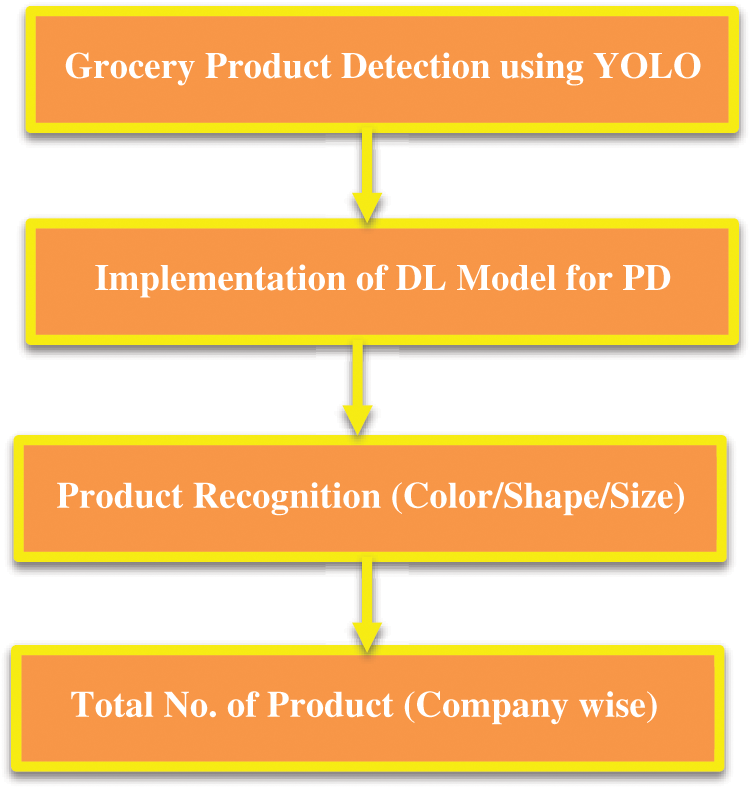
Figure 1: Proposed product recognition pipeline architecture
Process Flow:
Step 1: Product Detection – YOLOv5 is used to detect the products
Step 2: Product Recognition is done in the following steps for each product detected
Step 3: For the description of color, the color picker matches the color vocabulary of Naïve Bayes (NB).
Step 4: The color encoding and improvement is made by Fisher Kernel Method (FKM)
Step 5: Find the BoW histogram for color features
Step 6: For shape and size description, Gaussian shift is used
Step 7: Dirichlet function enhances the given shape and size feature
Step 8: Find the BoW histogram
Step 9: Concatenate the final vector considering the feature's weights and the image's threshold for a particular product.
Step 10: Based on the feature, identify the brand and update the count accordingly.
YOLO-v5 uses a sophisticated Convolutional Neural Network (CNN) for real-time object detection. In this algorithm, regions are derived by dividing the images, and the bounding boxes and every region probabilities are calculated. These bounding boxes are weighed based on the estimated probabilities. The method only needs a forward propagation to pass through the NN for the purpose of predictions so that it “just looks once” at the image. After a non-max suppression, the outputs of the known objects are obtained along with bounding boxes (which make sure that the object detection algorithm only recognizes each object once).
We obtain the supermarket shelves structure before recognizing an object, rather than looking for a brand logo anywhere on the image on the shelf. We use a top-down strategy rather than a bottom-up method at this point. We take advantage of the shape similarity between classes in this case. Tobacco products are unique in the sense that they feature the same warning pictures across brands, but there are numerous commonalities throughout classes. Various beverage brands, for example, have comparable bottle forms.
We assume that the products will never rotate out of a plane and have a comparable ratio of aspects to what we see on supermarket shelves. YOLOv5 has been used because of the resemblance.
The YOLOv5 architecture was created conceptually and is provided via a GitHub repository with earlier versions. As previously stated, Ultralystic enabled YOLOv5 are based on the PyTorch framework (an open-source ML library based on the Torch library), which is one among the most widely used in the AI community. However, because this is just a prototype design, researchers can tweak it to get the acceptable results for particular issues by layer addition, eliminating blocks, integrating new methods for image processing, modifying methods of optimization or functions of activation, and so on.
In YOLO [10], the bounding box data are represented as [Class, Center, Width, Height]. The centre point (Xcenter, R) can be computed through the minimum point (Xmin): Xcenter = Xmin + width2 Ycenter = Ycenter + height2 [11]. Have not named the bounding boxes because there is a problem of single object detection. However, because YOLO requires a label parameter, the bounding boxes must be labelled with the classes’ names. Because all bounding boxes are in charge of detecting wheat, they are labelled ‘0’ as because class numbers are zero-indexed (beginning at 0), the label ‘0’ symbolizes the wheat head.
Box coordinates must be regularized to a value between 0 and 1. As a result, Xcenter and width are split by picture width, while ycenter and height are divided by image height. At this, the redundant parameters are eliminated. Each column of data now corresponds to the unique image id, class, Xcenter, Ycenter, width, and height of the box bounded, respectively. Positive images contain items, while negative images are photographs that do not contain objects. Negative photos must have labelled text files associated with them for the YOLOv5 model to access them and use during training. These photographs have no boundary boxes since they do not contain any objects.
We quickly receive the products’ bounding boxes on shelves due to the product detection module executed on devices in real-time with low resources like smartphones. Figuring out the brand logo on each item is done in the next phase. We present a technique for determining shelf limits besides product and non-product segmentation of the image. This isn't a must-do, but it's a good idea. Counting and estimating the number of shelves can be done once we identify the shelf boundaries. The Y-axis histogram of the products’ projection is calculated to evaluate the distribution throughout the shelves. We apply a Gaussian filter to the signal to remove the noise caused by false positives. The peaks on this signal are automatically labelled as the location of products, and midpoints are labelled as a limit of shelves.
The Bag-of-Words (BoW) technique is preferred for brand recognition using logo images within the detected locations. The logo and the warning graphic are together present in the detected zone. Because the warning component of the image is consistent throughout brands, let us classify the initial 40% of the image starting from the topmost. In the same method, we only use the logo areas of the product photos during the training phase. The product detection module does not guarantee accurate products framing. It's possible that some of the logos won't be covered.
Furthermore, the shelf, the price tag, and other items can be partially ambiguous objects. As a result, the usage of local descriptors frequency is a real-world method. The logo image can be represented with a combination of shape and color information. One feature alone is sufficient to distinguish brands to some extent. While two brands have strikingly similar shapes, their colors may vary, or vice versa. As a result, combining color, shape, and size improves recognition results.
A set of d-dimensional vectors (one for each training image) is set as reference model TS = {TS1, TS2,…, TSn}. If f is the feature vector related to a candidate
where w is the window and s is the score, and a model's similarity score TSi is calculated as following Eqs. (1)–(3):
where:
si is the pre-processing stage score obtained
sm considers the number of matches among f and TS:
where sim(f, tsi) depends on the representation of features, the threshold value sThr is specific to a product and is based on a different validation set.
For shape and size description, Gaussian shift features are used, and for color description, a color chooser is used. We have sample histograms for every image: color, shape, and size.
3.3.1 Shape and Size Vocabulary
Latent Dirichlet Allocation (LDA) to BoW feature consisting of countable word histograms is assigned. The feature transform is likewise handled as a kernel function [12]. Although the Gaussian kernel is commonly used to represent feature vectors, some kernels are designed explicitly for histogram features, such as the χ2 kernel and the intersection kernel. Despite this, the kernel functions invariably necessitate kernel-based approaches, which are time-consuming to compute. As a result, the map of kernel features is suggested in [13], and this problem is avoided by explicitly describing (additive) kernels.
Gaussian Shift Theorem
In the Gaussian Shift Theorem, in the random variable Z, constant c, and function F for a standard Gaussian, we have the expectation, Eq. (4)
Given the decomposition of
Latent Dirichlet Allocation
Let's take a glance at the words that make up the name of the LDA model before we step detail into it. “Latent” refers to the model's discovery of “yet-to-be-found"/else “hidden” document's topic. ‘Dirichlet’ refers to the assumption of LDA that both the document's topic distribution and the topic's word distribution belong to Dirichlet distributions. ‘Allocation’ refers to the document's topics distribution.
LDA considers that documents are composed of words that aid to determine the subjects, and text is mapped with a topic list by allocating every word to a different topic. The probability of a word wj relating to subject Tk is represented by the value in each cell in the figure. The word and topic indices are denoted by ‘j’ and ‘k’, respectively. It's worth noting that LDA does not consider the word sequence and syntactic information. It considers documents to be nothing more than a word collection/BoW.
Finding the collection of words that reflect a specific topic is done either by selecting the top ‘r’ probabilities of Words/by setting a probability threshold and selecting probabilities of words that are more than or equivalent to the threshold value after probabilities are estimated. For example, if we concentrate on Topic-1 and choose the topmost four probabilities, assuming that the probabilities of the words not listed in the table are <0.012, Topic-1 can be represented as follows using the ‘r’ top probabilities words approach. If trees, mountains, rivers, and streams are represented by WORDK, WORD1, WORD2, and WORD3, then Topic-1 may be interpreted as “nature”.
The expected topics number in the documents is a significant input to LDA. If we set the expected topics to 3 in the previous example, each document can be represented as mentioned below, Eq. (6)
Topics 3 weights: Topic-1, Topic-2, and Topic-3 for a particular document are represented in the diagram above.
Algorithm For Shape And Size Feature Improvement Using Dirichlet
Step 1: The shape and size histogram features are regarded as probability mass functions
Step 2: Normalize the features using Hellinger normalization
Step 3: Induce the Dirichlet function to transform the histogram-based shape and size features
Step 4: send the shape and size features to the BoW Histogram
There are large number of Gaussian SIFT local descriptors where spatial grid points are densely extracted in 4-pixel steps at three different (16, 24, and 32 pixels) scales. We use the clustering of the NB algorithm to create 16,384 visual words from a million (transformed) Gaussian SIFT descriptors to select from the training photos at random. In three layers of the spatial pyramid, a picture is partitioned into sub-regions: 1 × 1, 2 × 2 and 3 × 1; The BoW features of the histogram are calculated for each sub-region and, after that, it is integrated with vector image features.
Color Picker: 2D f(x, y) matrix with M columns/N rows represents a digital image. The Hue, Saturation, and Value (HSV) model is one of several images that process color models. This model detects an object of a particular color and lowers outside light intensity. Six different hues such as brown, yellow, green, blue, black, and white were used to carry out the tests.
Color Processing: Numerous color models are available in color picture processing. Red Green Blue (RGB) model is extensively used in the monitor is a model which is used extensively. Three fragments of components of a color are used for image representation in this paradigm. HSV model, which has three components: hue, saturation, and value, is another model besides RGB. Hue can be defined as a measure of the wavelength found in the dominant color being received via the sight, whereas Saturation is the quantity of white light mixed in the hue.
The color space HSV is more instinctive than the color space RGB in terms of what people think about color. The matching colors change from Red to Yellow, Green, Cyan, Blue, and then Magenta before going back to Red as the hue (H) changes from 0 to 1.0. The related colors (Hues) convert from unsaturated (grey shades) to completely saturated (without white component) as saturation(S) varies from the range 0 to 1.0. The related colors are much brighter as the (V) value/brightness varies from 0 to 1.0. HSV's hue component lies in the 0° to 360° angle range, all resting around on a hexagon, as seen in Fig. 2. The color has RGB values of (0.5, 0.5, and 0.25); however it has HSV values of (30°, 3/4, 0.5). When a user wants to choose an interactive color, HSV is the right option, and when compared to RGB, it is simple for a client in getting the desired color.
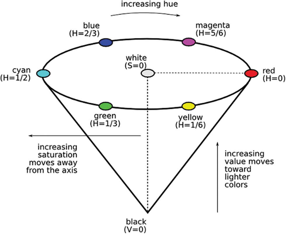
Figure 2: HSV representation of color-image
• HSV Distribution Process
Step 1-RGB TO HSV Conversion
We need to convert the image to HSV values for color isolation since HSV values are elementary to work with. Hue specifies the desirous color, saturation determines color clarity, and value determines the image's lightness in the HSV color representation. A moderate red color is specified by 0 on the wheel, while blue color is specified by 240. Instead of 0 to 360, the hue is a series from 0 to 1.
Step 2-Apply A Threshold Mask
Multiple masks are required in color isolation; a color, saturation, and value mask with low and high thresholds. A value of 1 is set to any pixel within these threshold limits and zero for the remaining pixels. A mask that obtains every red hue in the color wheel is applied in the algorithm. K-means clustering is time-consuming since it requires numerous iterations to acquire the desired color; color segmentation is used.
• Fisher Kernels On Visual Vocabularies
In Fisher kernels on visual vocabularies, visual word vocabularies are referred to in a Gaussian Mixture Model (GMM). X = {xt, t = 1…T} signifies the low-level feature vector set of an image, and λ signifies the parameter sets of the GMM.
The Fisher kernel considers order statistics, namely 1st and 2nd, when computing derivatives regarding means and standard deviations. The BoV produces an N-dimensional histogram with the vocabulary of size N, but the full gradient representation produces a vector of dimensionality (2D + 1) N – 1. This makes it possible for image characterization with too high vectors of dimensionality, in spite of vocabularies of only a few hundred words.
With Naïve Bayes, we cluster values of 3D color picker acquired from the photos of training to create a color vocabulary. Every cluster center in the vocabulary represents a visual word. The normalized frequency histogram represents every image in Vc dimensions after being provided with a set of Vc words that are visual. We practice a k-d tree structure to find the closest cluster center to assign a visual word's color value later. The labels are found with the help of FV. The picture representation of the Bag-of-Visual-words (BoV) in FV relies on visual vocabulary illustration in the intermediary. The visual vocabulary in a generative method is a probability density function indicated by ‘p’ that simulates the low-level descriptors’ image emission. GMsM is used to model the visual language, with each Gaussian representing a visual word. The FV is a BoV representation extension. An image is described by a vector of gradient created from a probabilistic generative model rather than the number of repetitions of each visual word. The log-likelihood gradient describes the parameters’ contribution to the process of generation.
GMM is used in the Fisher encoding to create a visual word dictionary. Consider a set of 2-D data points as an example of building a GMM. These points would represent local picture features compiled in reality.
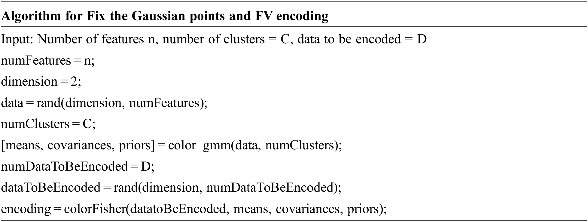
The FV representation of the data dataToBeEncoded is the encoding vector. We generate a new set of random vectors to encode using the FV Representation and the GMM. The colorFisher function is called along with the output of the color GMM function to obtain the encoding of FV of these vectors.
The histogram won't carry data about the image's spatial information because it is a numerical descriptor that sums the frequency of specific fundamental “patterns” throughout the entire picture. We partition the image into ‘r’ overlapping sections, encode every region independently (with its histogram), and later the features into a d = r * s vector with dimconcatenated dimensions to prevent the information from all of them. The proposed overlapping region indirectly strengthens the central region compared to the neighbouring ones that are frequently not completed or noisy (e.g., they may contain components from other goods).
The NB self-learning algorithm provides a method for approximation probability propagation in hybrid networks of Bayesian, in addition to clustering challenges. If the aim is probability propagation, this strategy can be competitive instead of developing a broad Bayesian network from a database. Zheqian 2021 [14] developed this notion, which depends on the simplicity of NB structures’ probability propagation. The condition distribution of every variable to other variables is represented by a mixture of marginal distributions in an NB model for a discrete class variable, with the number of components in the mixture equivalent to the volume of states of the class variable. The NB is trained with two kinds of a dataset. One of the models is trained with color features to recognize the products, and it is used to find the matches in the Color features, and another NB is trained with shape and size bag of words to identify the corresponding features.
Since the earlier steps may create numerous detections that are overlapping (window candidates) for the similar instance of the product, the last post-processing step is usually required in object detection; those detections have to be merged into a specific output, or false positives would be measured for several occurrences of the similar product. This point is crucial for overall detection performance, especially in strict valuation standards that need high overlap among the discovered object and the ground truth for detection is to be regarded correct. To make a single image out of overlapping pieces, assume that you know the full image size and the coordinates of each block within it.
Both horizontally and vertically, the blocks are evenly spaced. The point is that in the overlapping zone, a pixel in the output image should be assigned a value based on a weighted average of the overlapping blocks’ associated pixels.
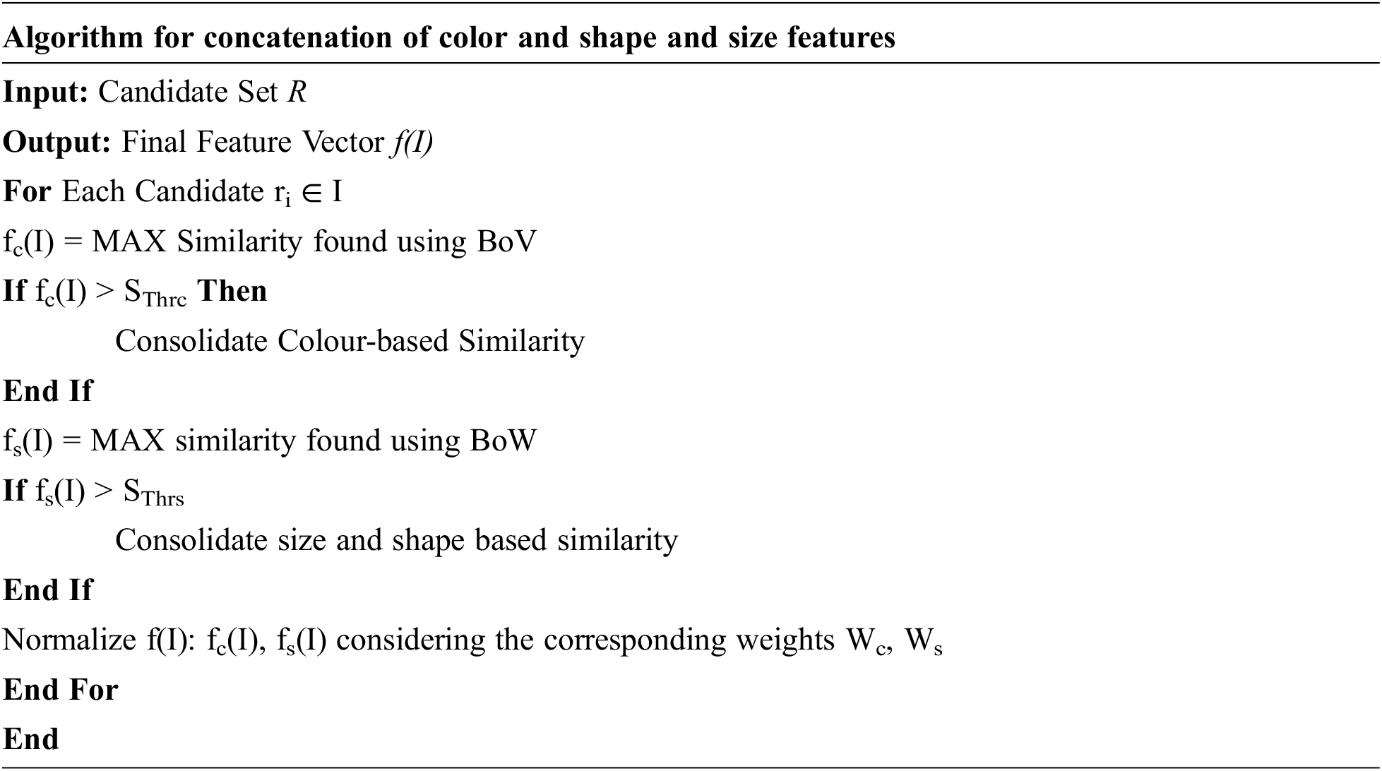
For each candidate r in the given set of images R, the maximum similarity feature fc(I) and fs(I) is found for color, shape and size separately, and it is compared with the corresponding threshold sThrc and sThrs for color, shape and size respectively. It is consolidated for the features if it is above the threshold value. Then it is normalized after considering the Wc and Ws as given.
To make a joint frequency histogram, we combine two normalized histograms. However, based on the cluster numbers, color vocabulary Vc and shape and size vocabulary Vs, one modality may outnumber the other if it is more significant in dimension. We use a weight learning strategy to solve this problem. Let us have wc and ws correspondingly represent the colour/shape descriptor weights.
The above Eq. (7) provides the Final Feature Vector f(I) by image I. Here, fc(I) and fs(I) denote the color and shape aspects, respectively. Since the final vector will be normalized, one free parameter will be learned. A single free parameter must be learned because the final vector will be normalized.
We examined using a benchmark that included photographs of store shelves. Various brands and items have different appearances. A typical store can sell hundreds of products, giving a detector a wide range of appearance changes between classes. On the other hand, sub-brands are frequently distinguished merely by minor modifications in packaging. The number of annoyances that detectors must get contended with is growing due to these modest appearance changes (e.g., spatial transformations, image quality, and occlusion). In terms of the amount and density of objects appearing in each image, the variety of its item classes, and, of course, the character of its scenes, SKU-110 K is quite different from the existing alternatives. There are 11,762 images in total, with an average of 147.4 goods per image. The number of image classes is 110,712.
The performance of product detection and brand recognition is assessed together. We also look into the impact of vocabulary size on color attributes and shape to find suitable features. Added Gaussian SIFT computation parameters are also investigated. P, the patch size and G, the grid spacing are two. The junction space between recognition and ground truth determines if a product is true positive. We agree with the detection that the internal intersection is over a given threshold, and the external intersection is under an actual threshold. In addition, single detection per product is accepted. As a result, detections due to overlapping reduce performance. The system can detect products on shelf photos with 98% recall and 84% precision. Figs. 3–5 give the accuracy percentage for selected vocabulary sizes, various patch sizes, Grid Spacing pixels and Number of words.
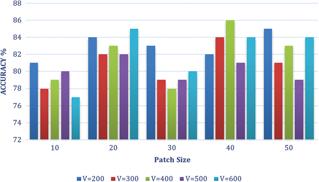
Figure 3: Accuracy % patch P vs. vocabulary V
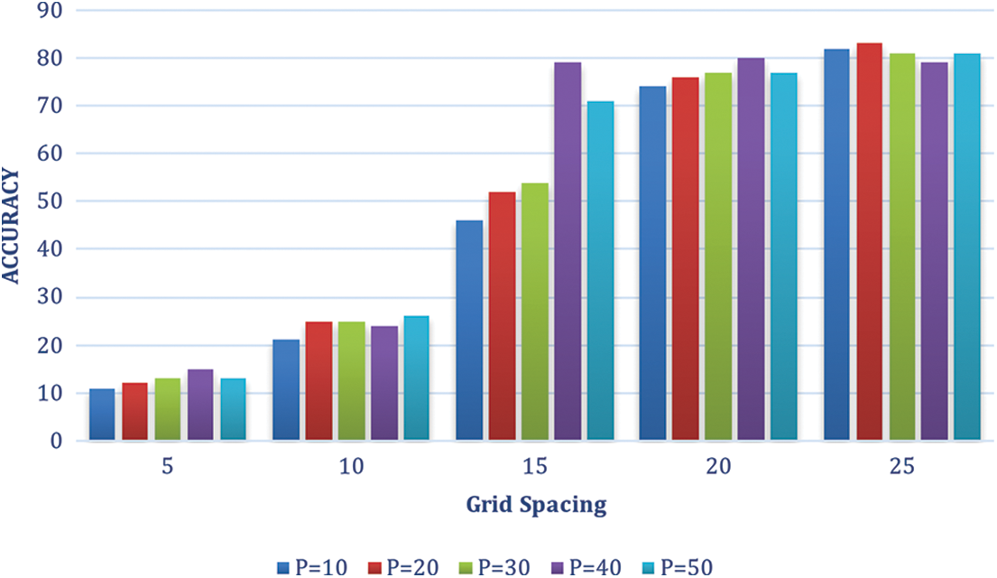
Figure 4: Accuracy % patch size P vs. Grid spacing pixels
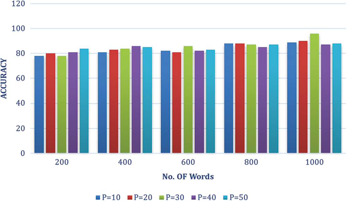
Figure 5: Accuracy % patch size vs. No. of words
The product detection recall rate is a promising finding. Each observed location should be classified as a brand by a comprehensive system. On the other hand, for the time being, we will not be dealing with products that do not fit into any of the categories. A system that deals with this issue can automatically ignore false alarms. Figs. 6 and 7 summarize the impact of the color vocabulary size and scaling. There is no evident regarding any changes in accuracy for varying vocabulary size and resizing values. On the other hand, color has a considerably limited vocabulary than shape because color has only three dimensions. For the various weights of color, the accuracy regarding feature level and score level is given in Fig. 8.
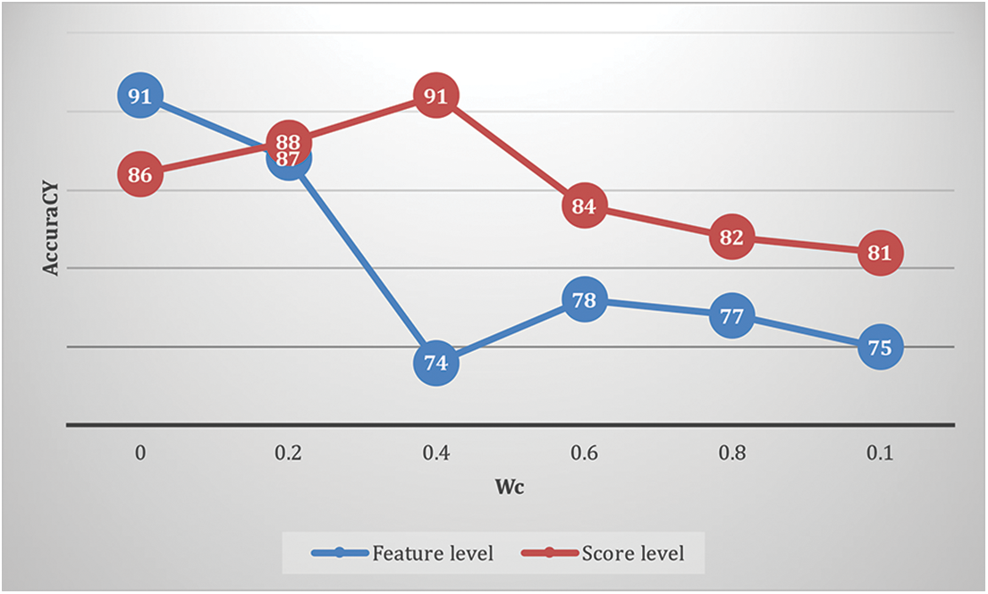
Figure 6: Accuracy using color features shape and size
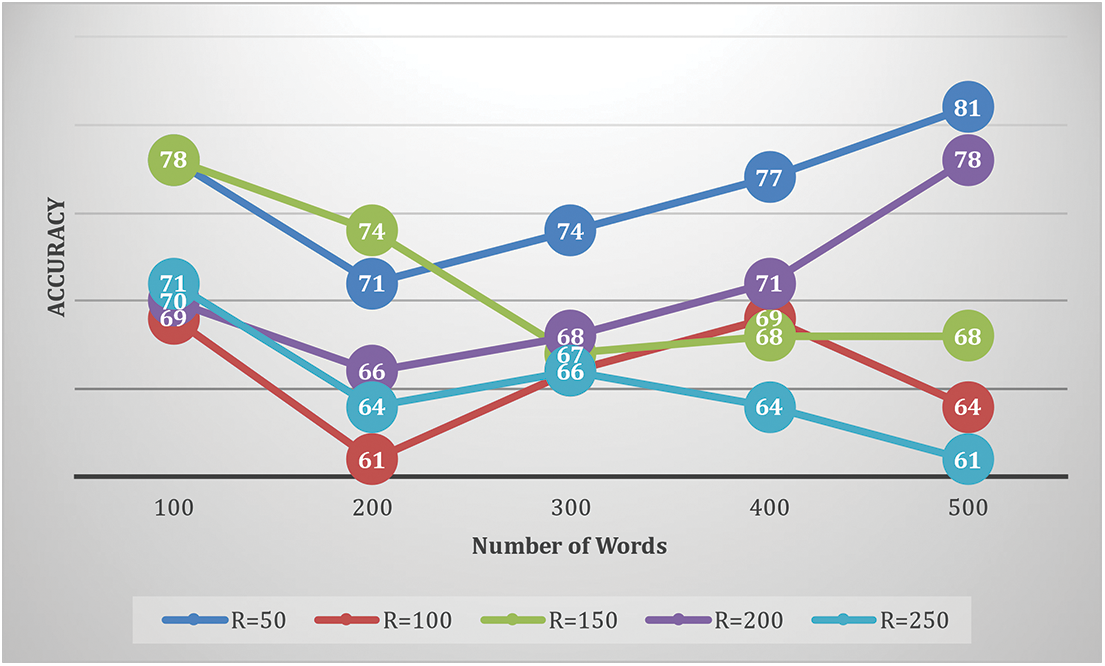
Figure 7: Accuracy using color feature for No. of words and No. of pixel R
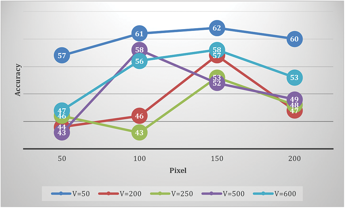
Figure 8: Accuracy using a color feature for various pixels and vocabulary size
For combination, we test at the level of features and scores. In feature-level fusion, very simple concatenation is used. Even though score-level fusion produces similar, or if not greater, accuracy for specific Wc values, we favor the level of feature fusion while scores are generated using margin distances, and accurate probabilities are not reflected always. When it comes to identifying these 10 product categories, we discover that the importance of shape outweighs the importance of color. Of course, the combined classification outperforms both individual classes in accuracy.
We compare our method Faster Region-based Convolutional Neural Network (RCNN) [15–20] and RetinaNet [21–25] algorithms for Average Precision (AP), Average Recall (AR) and Mean Average Error (MAE). The proposed algorithm performs better in AP, AR and MAR. The results are shown in Tab. 1 below.

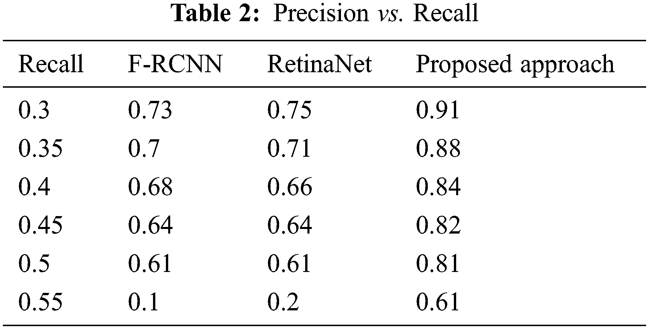
The Recall vs. Precision is compared for the proposed approach with Faster RCNN and RetinaNet algorithms [26–30]. Comparatively, the proposed algorithm performs better in precision and results are given if Tab. 2.
This paper describes a method for recognizing retail products on grocery shelves. The proposed module contains two distinct modules, and it can run independently. For product recognition, the color feature is also included, which helps in reducing the error date. It is helpful to distinguish between similar-looking logo which has different colors. We can achieve the accuracy percentage for feature level as 75 and score level as 81. Post-processing has improved efficiency. Using two vocabularies has improved the accuracy level. From the experimental results, it is shown that our proposed approach gives better performance.
Funding Statement: The authors received no specific funding for this study.
Conflicts of Interest: The authors declare that they have no conflicts of interest to report regarding the present study.
1. Y. Li, S. Wang, Q. Tian and X. Ding, “Feature representation for statistical-learning-based object detection: A review,” Pattern Recognition, vol. 48, pp. 3542–3559, 2015. [Google Scholar]
2. L. Zhang, Y. Wei, H. Wang, Y. Shao and J. Shen, “Real-time detection of river surface floating object based on improved RefineDet,” IEEE Access, vol. 9, pp. 81147–81160, 2021. [Google Scholar]
3. J. Sung, C. Ponce, B. Selman and A. Saxena, “Unstructured human activity detection from RGBD images,” in IEEE Int. Conf. on Robotics and Automation, Saint Paul, MN, USA, pp. 842–849, 2012. [Google Scholar]
4. M. George, D. Mircic, G. Sörös, C. Floerkemeier and F. Mattern, “Fine-grained product class recognition for assisted shopping,” in IEEE Int. Conf. on Computer Vision Workshop (ICCVW), Santiago, Chile, pp. 546–554, 2015. [Google Scholar]
5. T. Stahl, S. L. Pintea and J. C. V. Gemert, “Divide and count: Generic object counting by image divisions,” IEEE Transactions on Image Processing, vol. 28, no. 2, pp. 1035–1044, 2019. [Google Scholar]
6. M. Merler, C. Galleguillos and S. Belongie, “Recognizing groceries s using in vitro training data,” in IEEE Conf. on Computer Vision and Pattern Recognition, Minneapolis, MN, USA, pp. 1–8, 2007. [Google Scholar]
7. E. Goldman, R. Herzig, A. Eisenschtat, J. Goldberger and T. Hassner, “Precise detection in densely packed scenes,” in IEEE/CVF Conf. on Computer Vision and Pattern Recognition (CVPR), Long Beach, CA, USA, pp. 5222–5231, 2019. [Google Scholar]
8. M. Marder, S. Harary, A. Ribak, Y. Tzur, S. Alpert et al., “Using image analytics to monitor retail store shelves,” IBM Journal of Research and Development, vol. 59, no. 2, pp. 1–11, 2015. [Google Scholar]
9. E. Frontoni, A. Mancini, P. Zingaretti and V. Placidi, “Information management for intelligent retail environment: The shelf detector system,” Information, vol. 5, no. 2, pp. 255–271, 2014. [Google Scholar]
10. V. Nogueira, H. Oliveira, J. A. Silva, T. Vieira and K. Oliveira, “RetailNet: A deep learning approach for people counting and hot spots detection in retail stores,” in 32nd SIBGRAPI Conf. on Graphics, Patterns and Images (SIBGRAPI), Rio de Janeiro, Brazil, pp. 155–162, 2019. [Google Scholar]
11. M. Ondrašovič and P. Tarábek, “Siamese visual object tracking: A survey,” IEEE Access, vol. 9, pp. 110149–110172, 2021. [Google Scholar]
12. Q. Wang, L. Zhang, L. Bertinetto, W. Hu and P. H. S. Torr, “Fast online object tracking and segmentation: A unifying approach,” in Proc. IEEE/CVF Conf. Computer Visual Pattern Recognition (CVPR), Long Beach, CA, USA, pp. 1328–1338, 2019. [Google Scholar]
13. R. Ajoodha and B. Rosman, “Tracking influence between Naïve Bayes models using score-based structure learning,” in Pattern Recognition Association of South Africa and Robotics and Mechatronics (PRASA-RobMech), Bloemfontein, South Africa, pp. 122–127, 2017. [Google Scholar]
14. L. Zheqian, “Research on smart vending machine of gym under the concept of public service,” in Int. Conf. on Public Management and Intelligent Society (PMIS), Shanghai, China, pp. 62–65, 2021. [Google Scholar]
15. S. Chaudhary and S. Murala, “A Real-time fine-grained visual monitoring system for retail store auditing,” in 4th IEEE Int. Conf. on Image Information Processing (ICIIP), Shimla, India, pp. 1–6, 2017. [Google Scholar]
16. M. Stark, M. Goesele and B. Schiele, “Back to the future: Learning shape models from 3D CAD data,” Proceedings BMVC, vol. 2, no. 4, pp. 106.1–106.11, 2010. [Google Scholar]
17. L. Marchesotti, C. Cifarelli and G. Csurka, “A framework for visual saliency detection with applications to image thumbnailing,” in IEEE 12th Int. Conf. on Computer Vision, Kyoto, Japan, pp. 2232–2239, 2009. [Google Scholar]
18. S. Ren, K. He, R. Girshick and J. Sun, “Faster R-CNN: Towards real-time object detection with region proposal networks,” IEEE Transactions on Pattern Analysis and Machine Intelligence, vol. 39, no. 6, pp. 1137–1149, 2017. [Google Scholar]
19. X. Chen and J. Li, “Research on an efficient single-stage multi-object detection algorithm,” in IEEE Int. Conf. on Smart Grid and Electrical Automation (ICSGEA), Xiangtan, China, pp. 461–464, 2019. [Google Scholar]
20. T. Y. Lin, P. Goyal, R. Girshick, K. He and P. Dollár, “Focal loss for dense object detection,” IEEE Transactions on Pattern Analysis and Machine Intelligence, vol. 42, no. 2, pp. 318–327, 2020. [Google Scholar]
21. J. Hosang, R. Benenson, P. Dollár and B. Schiele, “What makes for effective detection proposals?” IEEE Transactions on Pattern Analysis and Machine Intelligence, vol. 38, no. 4, pp. 814–830, 2016. [Google Scholar]
22. J. LiJia and J. JiaFu, “Object detection method based on dense connection and feature fusion,” in 5th Int. Conf. on Mechanical, Control and Computer Engineering (ICMCCE), Harbin, China, pp. 1736–1741, 2020. [Google Scholar]
23. D. Yuan, X. Lu, D. Li, Y. Liang and X. Zhang, “Particle filter re-detection for visual tracking via correlation filters,” Multimedia Tools and Applications, vol. 78, no. 11, pp. 14277–14301, 2019. [Google Scholar]
24. X. Shu, D. Yuan, Q. Liu and J. Liu, “Adaptive weight part-based convolutional network for person re-identification,” Multimedia Tools and Applications, vol. 79, no. 31, pp. 23617–23632, 2020. [Google Scholar]
25. D. Yuan, X. Chang, P. Y. Huang, Q. Liu and Z. He, “Self-supervised deep correlation tracking,” IEEE Transactions on Image Processing, vol. 30, pp. 976–985, 2021. [Google Scholar]
26. T. Y. Lin, P. Goyal, R. Girshick, K. He and P. Dollár, “Focal loss for dense object detection,” IEEE Transactions on Pattern Analysis and Machine Intelligence, vol. 42, no. 2, pp. 318–327, Feb. 2020. [Google Scholar]
27. P. F. Felzenszwalb, R. B. Girshick, D. A. McAllester and D. Ramanan, “Object detection with discriminatively trained part-based models,” IEEE Transactions on Pattern Analysis and Machine Intelligence, vol. 32, no. 9, pp. 1627–1645, 2010. [Google Scholar]
28. J. Xiao, S. Zhang, Y. Dai, Z. Jiang, B. Yi et al., “Multiclass object detection in UAV images based on rotation region network,” IEEE Journal on Miniaturization for Air and Space Systems, vol. 1, no. 3, pp. 188–196, 2020. [Google Scholar]
29. X. Li, W. Wang, X. Hu, J. Li, J. Tang et al., “Generalized focal loss V2: learning reliable localization quality estimation for dense object detection,” in IEEE/CVF Conf. on Computer Vision and Pattern Recognition (CVPR), Nashville, TN, USA, pp. 11627–11636, 2021. [Google Scholar]
30. K. R. Jyothi and M. Okade, “Computational color naming for human-machine interaction,” in IEEE Region 10 Symposium (TENSYMP), Kolkata, India, pp. 391–396, 2019. [Google Scholar]
 | This work is licensed under a Creative Commons Attribution 4.0 International License, which permits unrestricted use, distribution, and reproduction in any medium, provided the original work is properly cited. |