A New Route Optimization Approach of Fresh Agricultural Logistics Distribution

Daqing Wu; Jiye Cui; Dan Li; Romany Mansour

doi:10.32604/iasc.2022.028780

1College of Economics and Management, Shanghai Ocean University, Shanghai, 201306, China
2Nanchang Institute of Technology, Economic and Technological Development Zone, Nanchang, 330044, China
3School of Business Administration, Shanghai Lixin University of Accounting and Finance, Shanghai, 201600, China
4Department of Mathematics, Faculty of Science, New Valley University, El- Karaga, 72511, Egypt
*Corresponding Author: Jiye Cui. Email: jguocui@163.com
Received: 17 February 2022; Accepted: 11 April 2022

Abstract: Under the fierce market competition and the demand of low-carbon economy, the freshness of fresh products directly determines the degree of customer satisfaction. Cold chain logistics companies must pay attention to the freshness and carbon emissions of fresh products to obtain better service development. In the cold chain logistics path optimization problem, considering the cost, product freshness and carbon emission environmental factors at the same time, based on the cost-benefit idea, a comprehensive cold chain vehicle routing problem optimization model is proposed to minimize the unit cost of product freshness and the carbon trading mechanism for calculating the cost of carbon emissions. The improved adaptive chaotic ant colony algorithm is used to perform calculation experiments on the model, and the feasibility and effectiveness of the model are analyzed through classic examples and actual cases, which proves the feasibility of the model and the effectiveness of the algorithm. This model enriches the logistics and distribution of cold chain optimization studies, and the research results supplement the impact of carbon prices on carbon emissions, emissions and customer satisfaction. Finally, there are some practical enlightenments for the provision of business management and government services.

Keywords: Fresh product; vehicle routing problem; carbon emission; cold chain logistics

With the continuous improvement of people’s happiness in life, the safety and quality of food have received more and more attention from consumers [1]. Some data from the relevant statistical departments of our country show that our country has more than 400 million middle-income groups, and this group is constantly expanding. As a result, people’s consumption demand is growing rapidly, and fresh products such as fruits and vegetables account for an increasing proportion of people’s daily consumption needs. More and more consumers are willing to buy better quality food at a higher cost [2]. In order to meet market demand, the cold chain logistics industry is developing rapidly. While controlling the cost of transportation, companies improve customer stickiness and enhance their competitiveness by improving the freshness of fresh products while reducing food waste. What’s more, some developments in recent years in some industries that use refrigerated trucks has also brought more severe environmental problems. At the 75th United Nations General Assembly in 2020, General Secretary Xi Jinping proposed that our country strive to achieve carbon peaks by 2030 and carbon neutrality by 2060. In the entire world’s carbon emissions, 14% of the carbon emissions are generated by transportation related industries, and more than 70% of the entire transportation industry’s carbon emissions are generated by road transportation [3]. The logistics transportation using refrigerated trucks has higher carbon emissions than those using ordinary vehicles. Therefore, controlling carbon emissions in the logistics transportation using refrigerated trucks is conducive to achieving carbon peak and carbon-neutral goals. At the same time, considering national policies and market demand, cold chain logistics companies for fresh products should not only pay attention to transportation costs, but also solve the two issues closely related to consumers’ lives, the freshness of food and the carbon emissions of distribution vehicles, so as to maintain economic and environmental performance and realize its corporate value.

The cold chain logistics transportation problem is essentially the Vehicle Routing Problem (VRP), which was proposed in 1959 by Dantzing et al. [4]. This is a vehicle optimal scheduling problem that satisfies different constraints and there have been many research results on VRP up to now. In the study of the VRP problem of cold chain logistics, the perishability of fresh products is a focus of scholars’ research. In order to solve the transportation problem of perishable goods, Shukla et al. [5] proposed a vehicle routing model with a time window with the total cost of transportation, deterioration, and fines as the goal, and used the artificial immune system to solve the difficult problem. Ma et al. [2] came up with a hybrid ant colony algorithm containing local search operators under the framework of perishable product distribution, which solved the problem of distribution service and time allocation with the purpose of maximizing profit. In order to optimize the logistics and distribution of fresh agricultural products using refrigerated trucks, Chen et al. [6] established a multi-compartment vehicle routing problem for fresh agricultural products with the goal of minimizing all costs in the entire delivery process, and solved and calculated it by introducing a method of combining neighborhood search strategy and particle swarm algorithm. Yao et al. [7] used ant colony algorithm to solve the distribution route optimization model that minimizes the total cost including cargo damage cost, and concluded that logistics distribution based on real-time road conditions and connection methods can effectively reduce distribution costs. Zhang et al. [8] set time and quality as satisfaction, and used them as the constraints of the cold chain distribution model, and compared them through the partial elite single parent genetic algorithm, and concluded that multiple models are more suitable for cold chain distribution scheduling. As the concept of environmental protection continues to deepen, the topic of carbon emissions is getting more and more discussion in academia, and academics have also begun research in the field of low-carbon cold chain logistics. Kang et al. [9] added carbon emissions as a cost to the total cost, and took the total cost as the goal of the fresh agricultural product distribution route optimization model considering carbon emissions, and combined the 2-opt local search mechanism to improve the ant colony algorithm to solve the problem and analyze the sensitivity of the parameters of the algorithm. Zulvia et al. [10] proposed a green vehicle routing model that considers operating costs, deterioration costs, carbon emissions and customer satisfaction, and designed an improved multi-objective gradient evolution algorithm, which verified the superiority of the algorithm by solving practical problems with the model and algorithm. Ren et al. [11] constructed a cold-chain vehicle path optimization model with minimum carbon emissions as the optimization goal based on customer satisfaction, and used an improved ant colony algorithm to perform simulation solutions, which proved that the model not only satisfies the enterprise economy but also meets social benefits. Liu et al. [12] built a vehicle path planning problem model under time-varying network with time window and freshness restriction with minimum freshness restrictions based on the perspective of both economic and environmental costs, and designed an adaptive and improved ant colony algorithm to solve the complicated question. In recent years, many scholars have begun to use different methods to study various derivative problems [13–19], such as the vehicle routing problem of electric vehicles, but they are still relatively rare in life, so this article will not discuss them for the time being.

There are two main problems in the existing research on vehicle path optimization of cold chain logistics distribution: (1) For the problem of cold chain logistics path optimization, on the one hand, many scholars study vehicle path optimization under static networks. On the other hand, many scholars focused on the optimization of carbon emissions in the distribution process, and they studied how to minimize the total cost of distribution as the goal in a theoretical scenario to rationally arrange the delivery route and loading sequence of vehicles, using heuristic algorithms, precise algorithms, and meta-heuristic algorithms solve similar path optimization problems. (2) ACO (ant colony optimization) is widely used to solve the VRP due to its good robustness and parallel characteristics. However, the global search ability of ACO is poor, in the initial stage of the algorithm, it is easy to fall into the local optimum due to the lack of path pheromone. As a result, the solution of the VRP can be further optimized and improved.

Aiming at the above two problems, based on the perspectives of economic cost and environmental cost, this research constructs a cost-benefit optimal mathematical model aiming at minimizing the average freshness cost. The model not only considers the decline of freshness of fresh agricultural products over time, but also introduces the measurement function of freshness of agricultural products and the measurement function of carbon emission rate. When using the algorithm to solve this problem, chaos theory is introduced, and an improved ant colony algorithm is designed which integrates the dynamic probability selection strategy and the pheromone update strategy. The effective information recorded in the iteration is used to guide subsequent operations, and based on multiple sets of experimental cases and traditional ant colony algorithms. The group algorithm is compared to verify the solving performance of the algorithm.

A distribution center needs to deliver fresh products to different customers. Each customer’s location and needs are different. All trucks must depart from the distribution center and return to the distribution center after serving customers. In the distribution process, not only the various costs must be considered, but also the carbon emissions and the freshness of the products delivered to the customers. The design of the distribution plan is carried out under the constraints of these restrictions and objectives.

1. There are a certain number of refrigerated trucks in the distribution center to serve customers, and the types of refrigerated trucks, refrigerating conditions, and load limits are all the same.

2. Data such as the number of customers, location, demand, service time for unloading at the door, and delivery time window are known quantities.

3. The same customer is distributed by only one refrigerated truck. A refrigerated truck can serve multiple customers under the condition of ensuring that the load limit is not exceeded. Only one vehicle is allowed to depart and arrive at each customer point.

4. The maintenance of the internal temperature of each refrigerated vehicle is only related to the refrigerant and has nothing to do with fuel consumption and carbon emissions.

5. Each customer has a fixed delivery time window. If the delivery vehicle does not deliver within the specified time window, a certain penalty fee must be paid.

6. The product maintains the maximum freshness in the distribution center. The freshness of the product begins to decrease by a certain percentage at the moment of departure of the delivery vehicle.

K : The total number of vehicles in the distribution center that meet the distribution requirements;

a : The maintenance cost per unit time of the delivery vehicle during the transportation stage;

b : The maintenance cost per unit time of the delivery vehicle during the loading and unloading stage;

tik : The time point when the delivery vehicle k arrives at the customer point i;

t0k : The time point when the distribution vehicle k departs from the distribution center;

tijk : The time for the delivery vehicle k from the customer point i to the customer point j;

si : The service time of the delivery vehicle unloading at the customer’s point i at the opening door;

u1 : The penalty cost for the delivery vehicle to arrive earlier than the time window;

u2 : The penalty cost for the delivery vehicle to arrive later than the time window;

Qij : The weight of the goods carried by the delivery vehicle when the customer point i goes directly to the customer point j;

The model [20] starts from the two perspectives of minimizing operating cost (C) and maximizing average freshness (AF), and it uses the ratio of operating cost to average freshness as the objective function. The objective function is shown in (1), and the decision variable is shown in (2).

When the vehicle k drives directly from the customer point i to the customer point j, that is, when the vehicle passes through the path (i, j), xijk is 1, otherwise xijk is 0.

Fixed costs generally include driver wages, vehicle maintenance costs, depreciation costs etc. and are only related to the number of vehicles used, which can be represented by (3).

x0jk means that the vehicle k departs from the distribution center to the customer point.

The cost of maintaining temperature refers to the refrigerant consumption in the refrigerated vehicle to keep the temperature in the compartment at a certain level. The rate of refrigerant consumption during the vehicle driving process and the waiting time is the same, which is lower than the rate of refrigerant consumption when the door is opened and unloaded. The maintenance cost can be represented by (4), and the waiting time is represented by (5).

The customer will agree on a time window ( ei , li ) with the distribution center, and the delivery vehicle will need to pay a certain penalty cost if it arrives earlier or later than the stipulated time, and there is no additional cost for arrival within the stipulated time. The penalty cost is represented by (6).

From the literature [21], it can be known that the fuel consumption cost and carbon emission cost are collectively referred to as the green cost. According to the fuel consumption, the load estimation method can be used to calculate. When the vehicle load M is delivered, the fuel quantity per unit distance of normal driving is shown in (7).

The fuel consumption rate per unit distance for normal driving is ρ0 when the delivery vehicle load is 0, and the fuel consumption rate per unit distance for normal driving is ρ∗ when the vehicle is fully loaded (load is ck ). The fuel consumption can be calculated according to the fuel consumption rate and distance under different loads. There is a certain linear relationship between carbon emissions and fuel consumption, from which the green cost can be calculated as shown in (8).

Among them, c is the oil price; γ is the environmental cost coefficient, that is, the product of the carbon tax and the carbon emission coefficient.

It can be seen from the literature that the freshness of a unit product during the distribution process can be represented by (9), and the average freshness delivered to the customer can be represented by (10).

Among them, T is the shelf life of the delivered product, ti is the time from the vehicle’s departure from the distribution center to the beginning of the service for the customer i, θ(ti) is the freshness of the product when the customer i receives its own needs.

The objective function of the model is expressed by (11), the minimum value of the total cost to the average freshness; (12) indicates that the delivery vehicles departing from the distribution center less than or equal to the total number of vehicles in the distribution center; (13) indicates that each delivery vehicle has a load less than or equal to the maximum load of the vehicle; (14) and (15) indicate that a customer is only allowed to be visited by one car once; (16) indicates that every car that departs from the distribution center finally returns to the distribution center; (17) indicates the continuity of time.

The vehicle routing problem studied in this paper is an N-P hard problem, which is usually solved by a heuristic algorithm. As a heuristic algorithm, ACO has positive feedback and strong robustness, but it has shortcomings such as long search time and prone to local optimization. In this paper, the distribution cost and product loss are taken as heuristic factors, and the adaptive function is given to calculate the transition probability, and finally the chaotic system is introduced to update the pheromone. In this way, the shortcomings of the ant colony algorithm can be overcome, so that the vehicle can reduce the cost during the transportation process, ensure the freshness of the fresh products, and better achieve the optimal cost and benefit.

As an important part of transition probability, heuristic factor is an crucial factor influencing the transfer of ants from one point to another. The research problem of this paper focuses on product quality and distribution cost, so two heuristic factors are designed to make the selection of the next point of ants affected by the total cost of movement and the damage of product quality during the movement. The heuristic factorial design is shown in Eq. (18). ηij is the reciprocal of the total delivery cost of the vehicle from customer i to j, θij is the reciprocal of the loss of product quality from customer i to j.

Among them, Cij is the total delivery cost of a vehicle from customer i to j, θ(tj) and θ(ti) is the freshness of the product when customer j and customer i receive the required products, respectively, and qj is the product demand of customer j.

The pheromone concentration and the two heuristic factors are assigned different degrees of importance δ , μ and ϵ , the transfer factor can be obtained. The transfer factor τijδηijμθijϵ can control the transfer probability of the vehicle so that the vehicle can deliver higher quality products to customers at a more reasonable cost.

The transition probability of the traditional ACO is easy to make the algorithm generate a local optimum. In order to solve this difficulty, this study introduces a random number r to select the transition probability, and selects from two transition methods through the generation of a random number. When r is greater than or equal to r0 , the vehicle will give priority to the customer with the largest transfer factor for delivery; when r is less than r0 , the roulette method is used to select the next customer point, and the vehicle will give priority to the customer with the largest transfer probability for delivery. The specific vehicle movement formula is shown in Eq. (19).

j={ argmaxl∈Nik[ τilδηilμθilϵ ],r≥r0;Use roulette to choose j according to probability Pijk:Pijk=τijδηijμθijϵ∑l∈Nikτilδηilμθilϵ,r<r0.(19)

Among them, Nik is a collection of other customer points that can be selected for service after vehicle k serves customer i.

As the number of iterations continues to increase, the pheromone concentration and the importance of the two heuristic factors also change. If δ , μ and ϵ are fixed constants, it is not conducive to getting rid of the drawbacks of the original algorithm. Therefore, the three are given as shown in Eq. (20). The different adaptive functions shown in the figure make the weight ratio between the three constantly change, and the transition probability can be adjusted adaptively [22].

Among them, iter is the number of iterations and maxiter is the maximum number of iterations.

Due to the positive feedback characteristic of the ACO, it can quickly find the approximate optimal solution, but it also makes it easier to fall into the local optimal solution and fail to jump out. The usual method is to combine the ACO with the local search algorithm. After the global solution is obtained, the optimized solution is searched locally, and the pheromone is updated according to the newly obtained optimized solution. In this way, the algorithm can move again near the optimized solution, which increases the probability that the algorithm searches for the global optimal solution. The chaotic disturbance is to use the random characteristics of the pure system to generate a pseudorandom variable within a range. Adding this random variable to the update of the pheromone can make it avoid the local optimum when looking for the optimal solution in the search process, which can improve algorithm search performance. To explore a more suitable delivery route, after all ants have gone through an iteration, the established route should be updated with pheromone. The pheromone update adopts the ant week model, and the pheromone change is the pheromone update constant divided by the total distance when the optimal goal is reached. The specific formula is shown in Eq. (21).

Among them, Q is the pheromone update constant, and Lk is the total distance to reach the optimal goal. When the pheromone is updated, the pheromone on the optimal path is volatilized and the pheromone change is added, as shown in Eq. (22); other paths that are not the optimal path only volatilize the pheromone, without adding other forms of information Supplement, as shown in formula (23).

Among them, ρ is the pheromone volatilization factor. λ is the coefficient that adjusts the mixed variable. zij is the mixed purity variable produced by the mixed purity system.

Step 1 Initialize the parameters. The parameters mainly include customer demand, distance, time window, total number of ants, and maximum number of iterations.

Step 2 Each ant selects and sorts all customer points in turn. Under the condition that the vehicle load limit is met, the state transition probability of each ant is obtained according to the formula, and the next access node is selected in turn until all nodes are traversed.

Step 3 Analyze the existing path of the ant and find the set of transferable customer points that meet the time window constraint and the load capacity constraint.

Step 4 Calculate the transition probability of the ant moving from the current position to each point in the set of transferable customer points, and determine the calculation formula of the transition probability according to the selection of random numbers.

Step 5 Find the next point according to the transition probability until all customer points are traversed. During the traversal process, if the time window or load capacity constraint is not met, return to the starting point and start again.

Step 6 After each ant has traversed all the points, calculate the total cost of this traversal, and compare the route of the optimal ant.

Step 7 Update pheromone. Update the pheromone concentration according to the improved pheromone update strategy.

Step 8 The algorithm ends the judgment. After the number of iterations reaches the specified maximum number of iterations, the iteration is terminated and the corresponding delivery route is output.

In order to verify the feasibility of the model, this paper uses the classic C101 example C101 in the VRPTW database for testing. Assuming that the number of ants is 10, the maximum load of the vehicle is 200 tons, the driving speed of the vehicle is 40 km/h, the fixed cost of each refrigerated truck is 200 yuan/day, and the maintenance cost of the transportation and loading and unloading process is 5 and 12 yuan/h, the penalty costs for early and late arrivals are 5 and 10 yuan/h, respectively. The fuel consumption rate when the vehicle is empty and fully loaded are 0.18 and 0.41 l/km, respectively. It is 5.41 yuan/l, the environmental cost coefficient is 0.008 yuan/l, and the shelf life of the product is 24 h. In order to effectively balance the relationship between the algorithm effect and the convergence speed [23], take 0.5 for r0 and set Q = 5. Solve the model according to the algorithm in this paper and C101 data, set the number of iterations to 20, run 10 times on the computer, and take the optimal result to get the minimum average freshness cost (MAFC) convergence graph and the vehicle optimal distribution plan (ODP) as shown in Figs. 2 and 3 shown.

It can be seen from Figs. 2 and 3 that in the 20 iterations of the algorithm, the average freshness cost of the target value tends to converge after three updates, and finally the average freshness cost of this optimal path is 12293 yuan, which can be derived from this article. The studied model can be solved through the operation of the classic database case C101, which has the computational feasibility of the model.

In order to verify the universality and effectiveness of the model and algorithm in this paper, the model and algorithm are used to solve different customer distribution examples. The test parameter design is the same as the previous section. C102, C104, C106, R102, R104, R106, RC102, RC104, RC106 nine examples of computer operation test 10 times, and the best results of all examples are recorded, the data test results are shown in Tab. 1, C104, R104, RC104 vehicle distribution map as shown in Fig. 4.

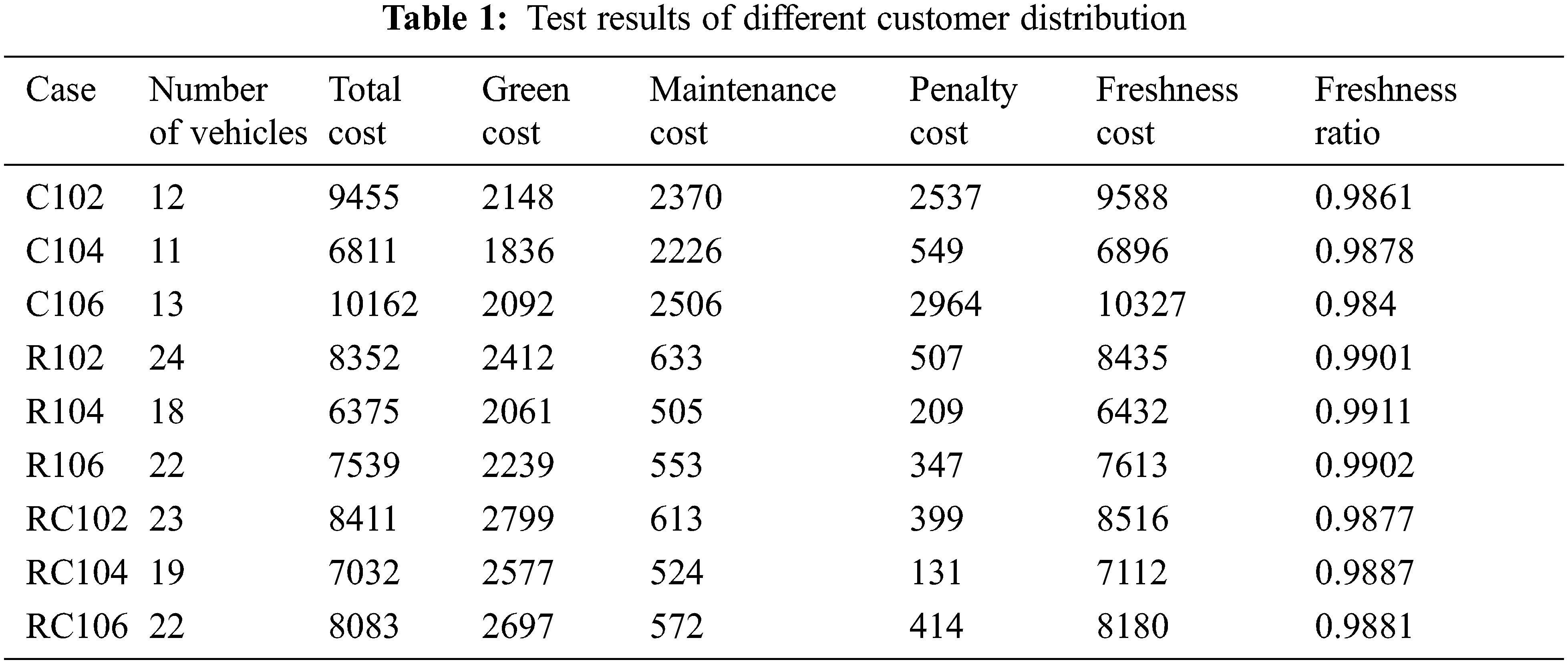
Figure 4: Vehicle distribution route diagram of different customer distribution examples

It can be seen from the test results that this model and algorithm can effectively solve different customer distribution examples and get their respective vehicle path planning. (1) It can be seen from Tab. 1 that the number of transportation vehicles in the C type calculation example is significantly less than that of the R type and RC type calculation example, but the maintenance cost and penalty cost during the transportation process are obviously higher. The customer locations of the type study are mainly distributed in several areas. The customer needs in the same area can be met by the same vehicle. The customer distribution of the R type and RC type studies is relatively random, and the distance between each customer is large. In order to maintain the total The cost is as low as possible, and only more vehicles can be sent for delivery. The transportation of multiple vehicles reduces the maintenance cost and penalty cost in the transportation process. (2) It can also be seen from Fig. 3 that in the C type example, the customers are more concentrated and the vehicle trajectory is relatively regular, while the R type and RC type examples have a wider distribution of customers, and the vehicle trajectory has no specific law. (3) In summary, different customer distributions will have a significant impact on the number of vehicles used, various costs, etc. Therefore, the different distribution of customers should be considered when optimizing vehicle distribution routes.

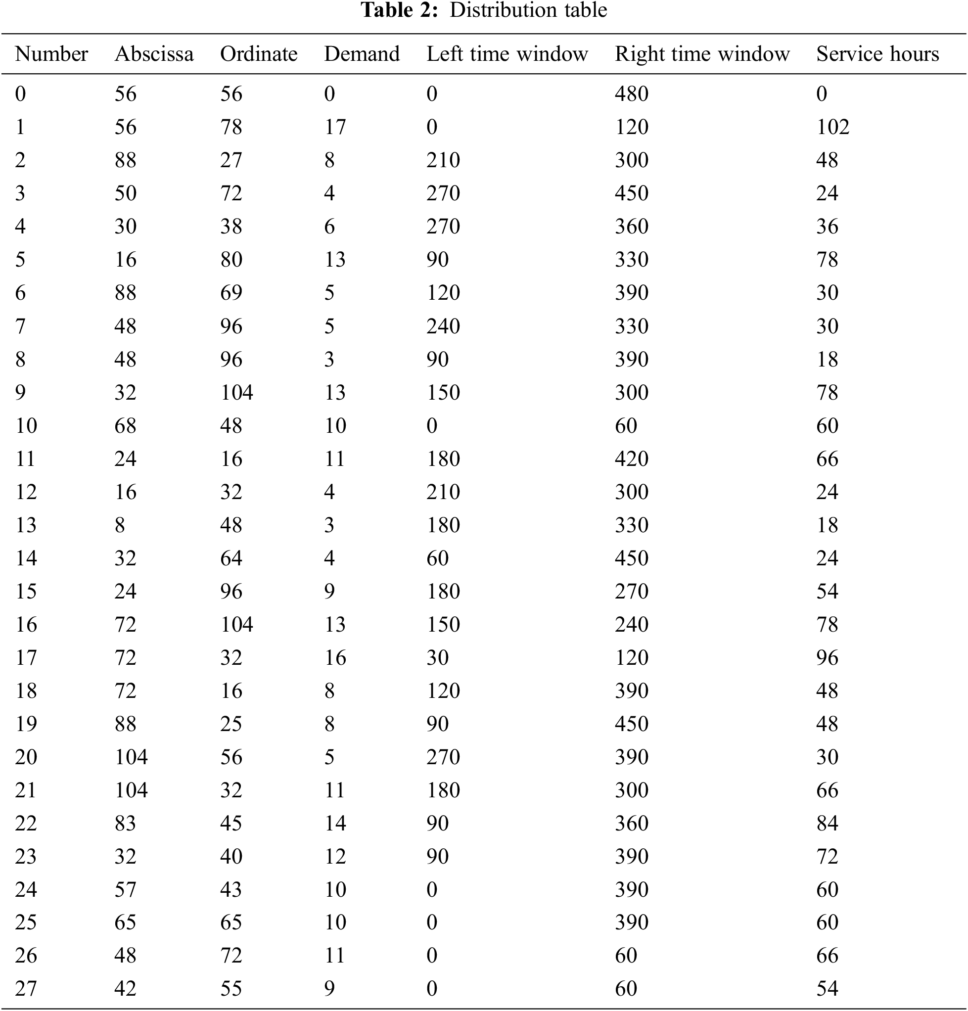
In order to further verify the practicability and effectiveness of the algorithm, this article uses examples for research and analysis. A distribution center provides distribution services to 26 customers in its vicinity. The location coordinates of the distribution center and each customer, the service time window, and the product demand and service duration of each customer are shown in Tab. 2.

Assuming that the number of ants is 10, the maximum load of the vehicle is 50 tons, the driving speed of the vehicle is 40 km/h, the fixed cost of each refrigerated truck is 200 yuan/day, and the maintenance cost of the transportation and loading and unloading process is 5 and 12 yuan/h, the penalty costs for early and late arrivals are 50 and 100 yuan/h, respectively. The fuel consumption rate when the vehicle is empty and fully loaded are 0.18 l/km and 0.41 l/km, respectively. It is 5.41 yuan/l, the environmental cost coefficient is 0.008 yuan/l, and the shelf life of the product is 24 h. In order to effectively balance the relationship between the algorithm effect and the convergence speed [23], take 0.5 for r0 and set Q = 5. Using the example data in Tab. 1, according to the model studied in this paper, the traditional ACO and the improved ACO proposed in this paper are used to program the solution respectively. The number of iterations is set to 20, and 8 random experiments are run on the computer. The results are shown in Tab. 3. For convenience, the number of vehicles delivered is denoted by N, the total cost is denoted by TC, the average freshness cost is denoted by AFC, the green cost is denoted by GC, and the freshness ratio is denoted by R. Through 8 random experiments, the results shown in the above table are obtained, from which the optimal results of the traditional ACO and the improved ACO are selected and compared, and the comparison table of the optimal results of the two algorithms can be obtained as shown in Tab. 4.

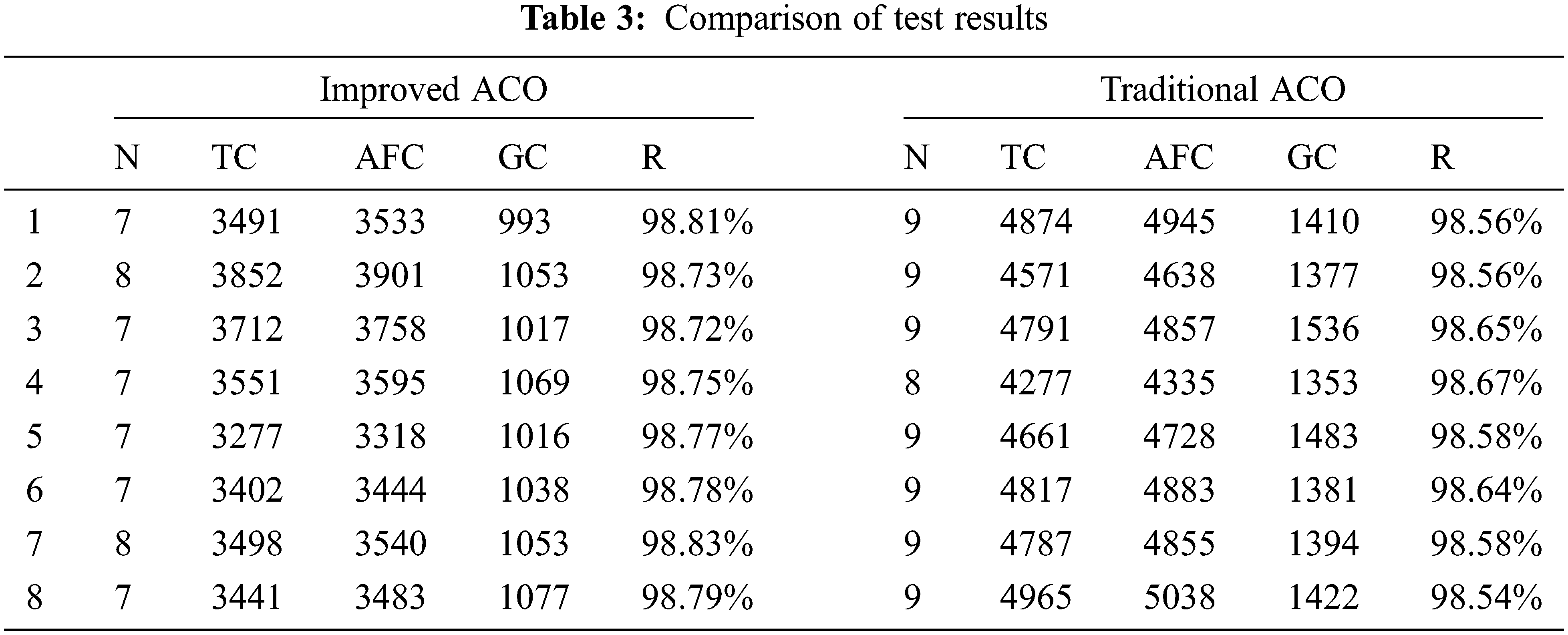
From the experimental results, for the cold chain logistics problem with the goal of minimizing the average freshness cost, the improved ACO proposed in this paper has better operating results than the traditional ACO. (1) It can be seen from Tab. 3 that in the test results of the improved ACO operation, although there are quantitative differences in the results each time, they are more superior than the results of the traditional ACO operation, especially in the required vehicles In terms of data and green costs, this is more conducive to the realization of the goal of green economy. (2) It can be seen from Tab. 4 that compared with the results of the traditional ACO, the operation result of the improved operation proposed in this paper reduces the number of delivery vehicles by 1 and reduces the labor cost. Although the freshness rate only increased by 0.1%, the average freshness cost was reduced by 23.4%, which means that the total cost was reduced by 22.2%, which reduced the company’s operating costs and improved the company’s benefits. Green costs have been reduced by 24.9%, reducing the consumption of environmental resources, saving energy and reducing emissions, and making it more low-carbon and environmentally friendly. (3) In summary, the improved ACO in this paper can speed up the convergence of the ACO and significantly reduce the costs incurred in the distribution process, which is more superior than the traditional ACO.

Common vehicle path planning problems are often studied based on the total distance traveled by the vehicle. Therefore, the goal of the minimum freshness cost and the minimum total travel distance proposed in this paper are compared and analyzed. The test parameters are consistent with the parameters used in the comparison of different algorithms in the previous section. Using the example data in Tab. 1, and according to the improved ant colony algorithm proposed in this paper, the models with the minimum freshness cost as the goal and the vehicle with the minimum total travel distance as the goal are carried out. Solve by programming, set the number of iterations to 20, and run 8 random tests on the computer. The test results are shown in Tab. 5. For convenience, the number of vehicles delivered is denoted by N, the total cost is denoted by TC, and the average freshness The degree cost is represented by AFC, the green cost is represented by GC, and the total distance is represented by TD. Because the objective function is different, it is inconvenient to compare the best results and only analyze the results of 8 trials.

Judging from the experimental results, the algorithm in this paper can solve the models of different targets and obtain satisfactory results. (1) It can be seen from Tab. 5 that under the same target, different test results are also different, but the model with the smallest freshness cost as the goal always has a smaller freshness cost and total cost, and the model with the total distance as the goal always has a smaller freshness cost and total cost. The distances are generally small, which shows the feasibility and effectiveness of the algorithm for the two target models. (2) It can also be seen from Tab. 5 that although the green cost of the model with the minimum freshness cost as the goal is low, it is not much different from the model with the total distance as the goal. The gap in the total cost is mainly concentrated in other delivery costs. In order to allow the vehicle to travel a shorter distance, more penalty costs need to be paid to achieve the goal. (3) In summary, companies should select optimization targets for vehicle path planning according to their actual conditions. The algorithm in this paper can effectively solve the vehicle path problem under different goals.

This paper conducts four different simulation experiments on the model by improving the ant colony algorithm, including the feasibility analysis, different customer distribution analysis, algorithm comparison analysis and different target analysis. The results of the simulation experiments show that:

1. The improved ant colony algorithm proposed in this paper can effectively reduce the cost of distribution, reduce the cost of carbon emissions, and reduce the use of vehicles.

2. The improved ant colony algorithm proposed in this paper can effectively solve the vehicle routing problem of different customer distributions of C type, R type and RC type.

3. The model proposed in this paper aiming at the minimum average freshness cost can effectively solve the vehicle routing problem under different objectives for fresh cold chain logistics enterprises.

With the continuous improvement of living standards, consumers’ demand for fresh products will continue to increase, and the effective way for fresh food companies to increase customer stickiness and enhance their own competitiveness is to improve the freshness of fresh products. From the perspective of environmental issues, this paper combines the minimization of enterprise operating costs and the maximization of the average freshness of delivered products, and proposes to model the cold chain logistics distribution path of fresh products with the goal of minimizing the unit freshness cost, which make companies guarantee greater product freshness at less cost. In order to better solve the model, this research improves the traditional ACO, takes the total cost and the loss of product freshness as heuristic factors, and randomizes the transition probability of ants, so that the algorithm effectively proposes a local optimum. The feasibility of the model and the effectiveness of the algorithm are verified through the classic VRPTW example. Finally, an actual case is used to compare the experimental results of different algorithms and different targets, and it is concluded that the model and target proposed in this article are superior to other models and targets.

Funding Statement: This research was funded by the China education ministry humanities and social science research youth fund project (No.18YJCZH192), the Applied Undergraduate Pilot Project for Logistics Management of Shanghai Ocean University (No.B1-5002-18-0000), the social science project in Hunan province (No.16YBA316).

Conflicts of Interest: The authors declare that they have no conflicts of interest to report regarding the present study.

References

Y. Cao, Y. M. Li and G. Y. Wang, “Study on the fresh degree incentive mechanism of fresh agricultural product supply chain based on consumer utility,” Chinese Journal of Management Science, vol. 26, no. 2, pp. 15, 2018.
Z. J. Ma, W. Yao and D. Ying, “A combined order selection and time-dependent vehicle routing problem with time widows for perishable product delivery,” Computers & Industrial Engineering, vol. 114, no. 1, pp. 101–113, 2017.
M. I. Piecyk and A. C. Mckinnon, “Forecasting the carbon footprint of road freight transport in 2020,” International Journal of Production Economics, vol. 128, no. 1, pp. 31–42, 2010.
G. B. Dantzig and J. H. Ramser, “The truck dispatching problem,” Management Science, vol. 6, no. 1, pp. 80–91, 1959.
M. Shukla and S. Jharkharia, “Artificial immune system-based algorithm for vehicle routing problem with time window constraint for the delivery of agri-fresh produce,” Journal of Decision Systems, vol. 22, no. 3, pp. 224–247, 2013.
J. M. Chen, N. Zhou and Y. Wang, “Optimization of multi-compartment cold chain distribution vehicle routing for fresh agricultural products,” Systems Engineering, vol. 36, no. 8, pp. 106–113, 2018.
Y. G. Yao and S. Y. He, “Research on optimization of distribution route for cold chain logistics of agricultural products based on traffic big data,” Management Review, vol. 31, no. 4, pp. 240–253, 2019.
Y. M. Zhang, Y. M. Li and H. O. Liu, “Research on VRP optimization of multi-type vehicle cold-chain logistics with satisfaction constraint,” Statistics & Decision, vol. 35, no. 4, pp. 176–181, 2019.
K. Kang, J. Han, W. Pu and Y. F. Ma, “Optimization research on cold chain distribution routes considering carbon emissions for fresh agricultural products,” Computer Engineering and Applications, vol. 55, no. 2, pp. 265–271, 201
F. E. Zulvia, R. J. Kuo and D. Y. Nugroho, “A many-objective gradient evolution algorithm for solving a green vehicle routing problem with time windows and time dependency for perishable products,” Journal of Cleaner Production, vol. 242, no. 1, pp. 1–14, 2020.
T. Ren, Y. Chen, Y. C. Xiang, L. N. Xing and S. D. Li, “Optimization of low-carbon cold chain vehicle path considering customer satisfaction,” Computer Integrated Manufacturing Systems, vol. 26, no. 4, pp. 242–251, 2020.
C. S. Liu, X. C. Zhou, H. Y. Sheng and L. Luo, “TDVRPTW of fresh e-commerce distribution: Considering both economic cost and environmental cost,” Control and Decision, vol. 35, no. 5, pp. 1273–1280, 2020.
Y. Xue, Y. Wang and J. Y. Liang, “A self-adaptive mutation neural architecture search algorithm based on blocks,” IEEE Computational Intelligence Magazine, vol. 16, no. 3, pp. 67–78, 2021.
Y. Xue, H. Zhu and J. Y. Liang, “Adaptive crossover operator based multi-objective binary genetic algorithm for feature selection in classification,” Knowledge-Based Systems, vol. 227, no. 5, pp. 1–9, 2021.
X. R. Zhang, W. F. Zhang, W. Sun, X. M. Sun and S. K. Jha, “A robust 3-D medical watermarking based on wavelet transform for data protection,” Computer Systems Science & Engineering, vol. 41, no. 3, pp. 1043–1056, 2022.
X. R. Zhang, X. Sun, X. M. Sun, W. Sun and S. K. Jha, “Robust reversible audio watermarking scheme for telemedicine and privacy protection,” Computers, Materials & Continua, vol. 71, no. 2, pp. 3035–3050, 2022.
D. Q. Wu and C. X. Wu, “TDGVRPSTW of fresh agricultural products distribution: Considering both economic cost and environmental cost,” Applied Sciences, vol. 11, no. 22, pp. 10579, 2021.
D. Q. Wu, Y. Liu, K. G. Zhou, K. Li and J. Li, “A multi-objective particle swarm optimization algorithm based on human social behavior for environmental economics dispatch problems,” Environmental Engineering and Management Journal, vol. 18, no. 7, pp. 1599–1608, 2019.
P. Mei, G. Ding, Q. Jin, F. Zhang and Y. Chen, “Reconstruction and optimization of complex network community structure under deep learning and quantum ant colony optimization algorithm,” Intelligent Automation & Soft Computing, vol. 27, no. 1, pp. 159–171, 2021.
G. Qin, F. Tao and L. Li, “A vehicle routing optimization problem for cold chain logistics considering customer satisfaction and carbon emissions,” International Journal of Environmental Research & Public Health, vol. 16, no. 4, pp. 576, 2019.
W. T. Fang, S. Z. Ai, Q. Wang and J. B. Fa, “Research on cold chain logistics distribution path optimization based on hybrid ant colony algorithm,” Chinese Journal of Management Science, vol. 27, no. 11, pp. 9, 2019.
Z. M. He, L. Zhang and W. Liang, “Vehicle path planning based on adaptive dynamic search ant colony algorithm,” Computer Engineering and Design, vol. 42, no. 2, pp. 9, 2021.
L. Li, S. X. Liu and J. F. Tang, “Improved ant colony algorithm for solving vehicle routing problem with time window,” Control and Decision, vol. 9, no. 5, pp. 102–106, 2010.

Intelligent Automation & Soft Computing DOI:10.32604/iasc.2022.028780
Article